Download

1 / 27
280 likes | 292 Views
Multi-Commodity Flow-Based Spreading in a Commercial Analytic Placer. Nima Karimpour Darav Andrew Kennings Kristofer Vorwerk Arun Kundu Physical & Logical Design Group. Outline. Background Motivation Implementation Details Experimental Results Conclusions. Background.

E N D
Multi-Commodity Flow-Based Spreading in a Commercial Analytic Placer Nima Karimpour Darav Andrew Kennings Kristofer Vorwerk Arun Kundu Physical & Logical Design Group
Outline • Background • Motivation • Implementation Details • Experimental Results • Conclusions
Background • Our FPGA hardware & software products are becoming increasingly complex: • 2004: ProASICPLUS • 2006: IGLOO • 2010: SmartFusion • 2012: SmartFusion2 • 2015: RTG4 • 2017: PolarFire • Increasing demand for both high-performance … • High-speed SERDES, DDR4, AXI buses. • FIR filters, CNNs, DSP-intensive tasks. • … and “group-based” design patterns: • Software region constraints. • Fixed cells (“obstacles”). • Tight timing budgets, and sophisticated timing constraints.
Motivation (1 of 2) Circuit Analytic Placer Timing, power, routability objectives. Clustering Lower-bound (LB) Placement Cluster Placement Goal of UB: preserve the LB objectives by not perturbing placement. Upper-bound (UB) Spreading Can Stop? Detailed Improvement The closer the UB to Full Legalization, the better the accuracy of timing predictions & decisions. Full Legalization Done
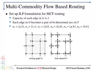
Motivation (2 of 2) Our UB strategy is based on network flow. • A grid can be imposed over the placement area. • Cells can be snapped into their nearest grid “bin”. • The bins are analogous, in many ways, to nodes in a flow problem. • The concept of flow can be used to push over-capacitated cells into under-capacitated sites.
High-Level Overview of the Spreading Algorithm (Part 1) Circuit + Architecture Construct Flow Network Assign cells to closest compatible bin Identify the overflowed bins Overflowed bins remain? No Yes End Establish limit on amount of movement For each bin, calculate the set of augmenting paths for the bin using BFS, then sort by cost Next bin All bins explored For each path, move cells along path
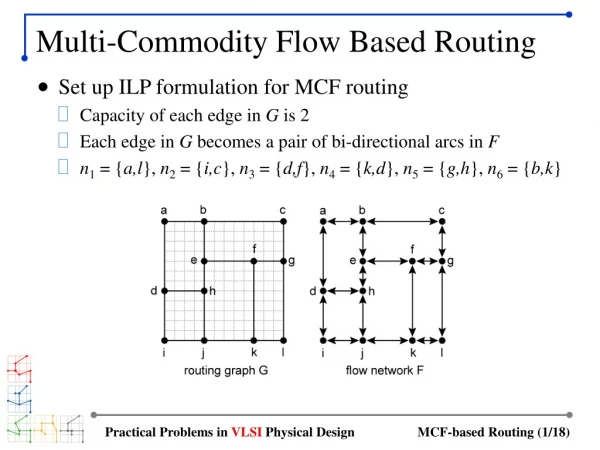
Step 1: Build the Flow Network (2 of 6) DSP Flow Network URAM Flow Network zoom-in … LSRAM Flow Network 4-direction connections
Step 1: Build the Flow Network (3 of 6) DSP Flow Network URAM Flow Network LUT (and Carry) Network LSRAM Flow Network Fused Flow Network
Step 1: Build the Flow Network (4 of 6) • In Microsemi’s FPGA products, non-carry LUTs can occupy locations within the URAM, DSP, and LSRAM sites, if those sites are unused. • This is referred to as using “shadow logic”. • Good for logic utilization. • Let’s see how this is supported… Distinct grids lend themselves to a convenient problem separation. This may be the case for some FPGA architectures… LUT (and Carry) Network
Step 1: Build the Flow Network (5 of 6) This required us to support a notion of “compatibility” to model cell-to-site legality. The LUTs need to be connected to the nearest URAM, LSRAM, and DSP sites because of the ability to occupy shadow locations. URAM Flow Nodes LSRAM Flow Nodes DSP Flow Nodes LUT Flow Node Fused Flow Network
Step 1: Build the Flow Network (6 of 6) Region1 Region constraints impact “compatibility”. Region2 URAM Flow Nodes LSRAM Flow Nodes DSP Flow Nodes LUT Flow Node The regions require different connections vs. previous slide. Fused Flow Network
High-Level Overview of the Spreading Algorithm (Part 2) Circuit + Architecture Construct Flow Network Assign cells to closest compatible bin Identify the overflowed bins Overflowed bins remain? No Yes End Establish limit on amount of movement For each bin, calculate the set of augmenting paths for the bin using BFS, then sort by cost Next bin All bins explored For each path, move cells along path
Step 2: Find Augmenting Paths (1 of 4) • Each augmenting path is a queue of bins whose first element is the overflowed bin. • While traversing bins using the BFS, partial paths are costed and saved into the queue. • The BFS is repeated until the queue of potential path choices is emptied or the total demand provided by the identified paths can sink the source bin. URAM Flow Nodes LSRAM Flow Nodes DSP Flow Nodes LUT & Carry Flow Nodes First Level Search
Step 2: Find Augmenting Paths (2 of 4) • A valid augmenting path starts with the supply node and ends with a sink node. C1 C2 C3 Suppose that these are carry chain LUTs whichare in overfilled LUT locations. In Microsemi’s FPGA, these cells can only be placed in (non-shadow) LUT locations. C4 C5 Valid Path
Step 2: Find Augmenting Paths (3 of 4) • A valid augmenting path starts with the supply node and ends with a sink node. • For adding a node into the end of path (compatibility conditions): • There must be at least one object in the source node with the same color as the destination node. C1 C2 C3 A bin is compatible with an object iff the object is not in a region constraint, or the region-color of the object is included in the region-color vector of the bin; and, the object can be legally placed into the bin of the corresponding type. C4 C5 Invalid Path
Step 2: Find Augmenting Paths (4 of 4) • A valid augmenting path starts with the supply node and ends with a sink node. • For adding a node into the end of path (compatibility conditions): • There must be at least one object in the source node with the same color as the destination node. • There must be at least one object from the source node to the destination node that must : • Not violate the max movement constraint. • Be allowed to be placed at the destination node. C1 C2 C3 C4 C5 Non-carry LUT; can go into DSP shadow location. Valid Path
Step 3: Move the Cells (1 of 3) • For a given augmenting path: Source Bin Sink Bin
Step 3: Move the Cells (2 of 3) • For a given augmenting path: • Loop until there are no bins left unexplored in the path… • Pop & examine the last bin from the path. • Choose the cell, in the bin, which is closest to & compatible with the sink. • Move the cell. • Update sink to the current bin. Sink Bin
Step 3: Move the Cells (3 of 3) • For a given augmenting path: • Loop until there are no bins left unexplored in the path… • Pop & examine the last bin from the path. • Choose the cell, in the bin, which is closest to & compatible with the sink. • Move the cell. • Update sink to the current bin. No newly-overflowed bins are created.
Experimental Results (1 of 5) • Conducted on a suite with: • 557 designs which we have used internally for benchmarking for many years. • A variety of sizes and design utilizations. • A variety of timing constraints. • Each design was placed into the smallest available PolarFire die which could fit it. • Each design was run with 5 different starting seeds, and averages reported here. • The placer was set to optimize the timing as best as it could (i.e., don’t stop early). • Timing is estimated using the pre-routing timing estimator embedded in the placer. • Results are compared after analytic placement, to our previous well-tuned approach based on geometric spreading.