y = p x 1 vector of responses

4. y= α + Γx+ Βy + ζ Φ = cov (x) = q x q matrix of covariances among xs y = p x 1 vector of responses α = p x 1 vector of intercepts Ψ = cov (ζ) = q x q matrix of covariances among errors Β = p x p coefficient matrix of ys on ys Γ = p x q coefficient matrix of ys on xs x = q x 1 vector of exogenous predictors ζ = p x 1 vector of errors for the elements of y Structural Equation Modeling:A Network Modeling Framework (a) the observed variable model 4

5. η = α + Γξ+ Β η + ζ x = Λxξ + δ y = Λyη + ε (b) the latent variable model where: η is a vector of latent responses, ξ is a vector of latent predictors, Β and Γ are matrices of coefficients, ζ is a vector of errors for η, and α is a vector of intercepts for η and: Λx is a vector of loadings that link observed x variables to latent predictors, Λy is a vector of loadings that link observed y variables to latent responses, and δ and ε are vectors are errors Estimates can be obtained either using likelihood or Bayesian methods. Equations can be hierarchical. 5

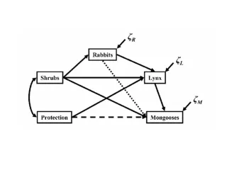
6. Hypothesized Probabilistic Network x1 x2 y1 tests for conditional independence ? ? y2 A Graphical Modeling Perspective In network models, each directed pathway between two variables, simple or compound, represents a different process.

7. topographic wetness plant species richness - + - topographic wetness herbaceous biomass plant species richness SEM Perspective: The concept of mediation what do we think the causal link might be? Hypothesize that wet areas produce taller grasses, which reduces richness So, we might postulate: If the second model holds, herbaceous biomass explains (mediates) effect of topographic wetness on plant richness. Note topographic wetness drops out of univariate model when the mediating variable(s) are present. If the second model does not hold, this implies another process is operating.

8. (A) (B) Environmental factors Phylogenetic distance Environmental factors Phylogenetic distance Grass species richness Trait distance Grass species richness Trait distance (C) (D) Environmental factors Phylogenetic distance Environmental factors Phylogenetic distance Grass species richness Trait distance Grass species richness Trait distance

9. Structural equation meta-model Water availability Rainfall - PET Moisture Drought index Disturbance Fire Rainfall concentration Fire frequency Soil fertility Percent sand Soil Biomass production Organic carbon Woody Biomass Tree biomass Minimum temperature Temperature Maximum temperature Climatic growing conditions

10. Results Large-scale Influences Landscape Curvature Local-scale Interactions - 0.45 - 0.30 Distance to Rivers 0.34 R = 0.67 2 0.29 - 0.40 Topographic Herbaceous Hotspot Wetness Index Biomass 0.30 - 0.50 - 0.17 Leaf Nitrogen Rainfall - 0.29 0.14 - 0.46 - 0.48 0.32 Soil Fertility Leaf Sodium 0.15 0.27 Leaf Magnesium

11. Large-scale Influences Local-scale Interactions Distance to Rivers Topographic Herbaceous Hotspot Wetness Index Biomass Leaf Nitrogen Rainfall Soil Fertility Leaf Sodium Leaf Magnesium We can consolidate paths if we wish. Landscape Curvature - 0.45 - 0.30 0.34 R = 0.67 2 0.29 - 0.40 - 0.50 - 0.17 0.45 - 0.29 N - 0.46 - 0.48 0.32 0.27

12. env. growing conditions biomass soils par ratio disturbance plant species richness species pool

13. env. growing conditions biomass soils par ratio disturbance plant species richness species pool

15. - Disturbance (grazing/fire) - Soils - Non-linear effects - Hierarchical design (plots within sites) p = 0.85