Download
1 / 41
430 likes | 575 Views
Advanced Research Methods: Regression Analysis Theory and Modeling By Erlan Bakiev, ph. D. . Faculty and Text. Textbook: Keith, T. Z. , (2006). Multiple Regression and Beyond. Pearson Montgomery, Peck, and Vining, Introduction to Linear Regression Analysis , 4th ed., 2006.

E N D
Advanced Research Methods:Regression Analysis Theory and ModelingBy Erlan Bakiev, ph. D.
Faculty and Text • Textbook: • Keith, T. Z., (2006). Multiple Regression and Beyond. Pearson • Montgomery, Peck, and Vining, Introduction to Linear Regression Analysis, 4th ed., 2006
Lecture Outline • Overview of Regression Analysis • Example • Guidelines for Group Project (due week 5 class)
Goals of Today’s Lecture • What is Regression analysis • Introduction to the most widely used statistical models • Linear regression • Logistic regression • How these models are used to analyze data and inform decisions • When different models are appropriate • How to fit, interpret, and assess different models • Practice with different data sets
A Note on SPSS • SPSS stands for Statistical Package for the Social Sciences and it is one of the most widely used programs for statistical analysis in social sciences. • Widely used by market researchers, health researchers, survey companies, government, education researchers, marketing organizations and others • User Friendly • You will use a basic set of commands for model fitting • Current version of SPSS is 18
Regression Analysis • Regression analysis is a statistical tool for the investigation of relationships between variables • İnvestigator seeks to understand the causal effect of one variable upon another, for example • the effect of a price increase upon demand, • the effect of changes in the money supply upon the inflation rate.
Types of Regression Models • Two types of regression models • Linear regression • Simple linear regression (continuous Y, one X) • Multiple linear regression (continuous Y, several Xs) • Logistic regression • Binary Y, several Xs • Linear regression forms the basis for understanding most regression techniques
Explore the Data Graphically Select a Tentative Structure Estimate the structure and its uncertainty Assess the plausibility of the tentative structure Use the estimated structure for your inferences (suitably qualified by the estimated uncertainty) Steps in a Regression Analysis
Simple Regression • Regression analysis with a single explanatory variable is termed “simple regression.” • Ex: Education income relationship • I = α + βE + ε α = a constant amount (what one earns with zero education); where • β = the effect in dollars of an additional year of schooling on in- come, hypothesized to be positive; and • ε = the “noise” term reflecting other factors that influence earn-ings.
Multiple Regression • İt is a technique that allows additional factors to enter the analysis separately so that the effect of each can be estimated.” • Simultaneously several independent variables can influence a dependent variable. • Ex: İnfluence of Education and experience on income • The model is as follows: I = α + βE + γX + εwhere “γ” is expected to be positive
Model-Based Data Analysis • Data sets consist of a set of observations • Each observation contains • One dependent variable (“Y”) • One or more independent variables (“Xs”) • We want to determine if there is a structure to the data set • Relationship between the response and one or more predictors
Response = structure(predictors) + “error” • Structure • Varies from observation to observation • Function of predictors • Systematic, deterministic • “Error” • The error of a sample is the deviation of the sample from the (unobservable) true function value.
Modeling Process • Fitting a model then requires: • Selecting a tentative structure • Estimating the structure and its uncertainty • Typically as statistics and their sampling distributions • Assessing plausibility of the choice of structure • Model diagnostics
Characterizing the Relationship BetweenTwo Variables • Outline • Types of variables • Correlation • Graphical Methods • Linear Regression
İndependent and Dependent Variables • Each observation has two parts: dependent Y and one or more independent Xs • We are interested in the relationship of X and Y • At a minimum, X and Y vary together • X and Y are associated • Statistical relationship does not imply causation Gujarati, D.N. (2003). Basic Econometrics, International Edition - 4th ed.. McGraw-Hill Higher Education. pp. 22-24. ISBN 0-07-112342-3.
Examples • X: income Y: consumption • X: parents’ SES Y: education level • X: education level Y: income • X: range to target Y: probability of hit/kill • The statistical methods we will study establish association • Association does not entail causality
Types of Variables • Continuous: variable can take any value in a (possibly infinite) range • Money, height, blood pressure, weight • Discrete: variable takes on a countable set of numerical values (often finite and small) • People in a queue, hits on a target • Ordinal: Variable has a finite set of non-numeric, but ordered values (categorical) • Level of schooling, rating • Nominal: Variable is finite, non-numeric, non-ordered • Religion, gender
Methods of Examining Relationships • Method X Y • Simple Regression continuous continuous • Multiple Regression continuous,discrete continuous • Logistic Regression continuous,discrete nominal • Other combinations are possible • These methods form the foundation of most other methods
Continuous X, Continuous Y • Simplest case • Correlation • Closely related to simple regression • Widely used in some substantive areas to characterize association • Graphical methods • Essential exploratory and diagnostic tool
Correlation • Definition • Attributes • Measures how X and Y vary together linearly • Scale-free • Ranges from –1 to +1 • Zero correlation is not necessarily independence • Note that this is pure association, no specification of response/dependent and predictor/independent variables
Problems with Correlation • Correlation is a single number summary of association • But • Outliers can dominate the value (it is not robust) • Zero correlation does not mean no relation • By itself, it does not allow the prediction of Y from X • This is usually of interest
Graphical Methods: Two-Way Scatterplot(1993 Car Data) infile _skip(11) EngSiz _skip(12) Wt _skip(1) using 93cars.dat scatter EngSiz Wt, ytitle("Engine Size (l)") xtitle("Weight (lbs)")
Linear Regression • In simple linear regression, we use the following model for the expected value of y given x: • E(y|x) = β0 + β1x • Relationship characterized by two numbers • Straight line • Wide applicability in practical situations • Many relationships approximately linear (or can be made so) • Forms the basis for more sophisticated analysis
The “Best” Straight Line • How do we construct the best line? • Some ideas • Minimize sum of distances from each Y to the line • Minimize sum of absolute values of distances from each Y to the line • Minimize sum of squared distances from Y to the line,
Regression Line for Car Data regress EngSiz Wt predict pengsiz scatter EngSiz Wt, ytitle("Engine Size (l)") xtitle("Weight (lbs)") || line pengsiz Wt, clc(black) EngSiz = -1.90 + 0.0015 Weight
Interpretation of Coefficients • In many applications we are interested in the coefficients directly • β1 is the change in expected value of y for a unit change in x (slope) • β1 = 0 means that x is not related to change in mean of y • β0 is the value of E(y) for x=0 (intercept) • Very often of little interest because reflects choice of origin • Often outside range of x data values
What We Need to Have to Do Inference • Construct 95% confidence interval for the slope • Get p-values for the t-statistic • This will allow us to state whether there is a statistically significant association between the independent and dependent variables • Test the hypothesis that β1 = 0 • SPSS, of course, does the arithmetic • In statistical significance testing, the p-value is the probability of obtaining a test statistic at least as extreme as the one that was actually observed, assuming that the null hypothesis is true. The lower the p-value, the less likely the result is if the null hypothesis is true, and consequently the more "significant" the result is, in the sense of statistical significance.
What does it mean to “explain” variation? • General idea • Want to assess whether the regression line “explains” the data better than simpler alternative models • Variation left after model fit is “unexplained” • R2 indicates what percent of variability in Y is accounted for by the regression model • Some properties of R2 • 0 R2 1 • R2=0: Regression line is horizontal • R2=1: Data fits perfectly on regression line
Multiple Regression Models • Extension of simple regression: • Together the βi are called the regression coefficients
In Policy Analysis Applicationsİndependent Variable Are Very Important • İndependent/ Categorical / Dummy Variables • Often at least part of our data is qualitative • Subject is male or female • Location is urban or rural • Others include ethnic group, insured vs. uninsured, high-school vs post-high school • Etc., etc., etc. • In much of the modeling in health most of the variables are qualitative • We need to generate the 0,1 indicators
Will LM Approach Work for Other Types of Data? • Suppose we have 0,1 data • Success/failure, die/live, leave military/stay, ... • Suppose we want to link p with covariates (age, income, disease, etc.)? • Least squares won’t work nicely … let’s take a look!
Example • We want to know whether the presence of CHD is related to age. • If we take a group of people of a given age • What is the fraction that have CHD? • Equivalently, what is the probability that a person of a given age has CHD? • We expect the probability to depend on age.
Linear Regression on 0,1 CHD Data Fitted values are out-of-range
Why A Different Type of Regression? • Logistic regression is the most commonly used generalization of multiple linear regression • Output data is categorical with 2 categories • Categorical: no metric, no order • Usually coded as 0/1 • Terminology: failure/success • Typical examples: dies/lives, does not/does have condition, does not/does marry, etc. • As we’ve seen, linear regression can be inappropriate
Interpretation • A year increase in age means that one is 11% more likely to have CHD than someone a year younger • But the probability that you have CHD is much different depending on age • Logistic regression is often used to see how much additional risk is contributed by some risk factor (e.g. smoking) • The coefficient shows how much the risk factor increases your chances of having some condition • But the probability may still be small
Group Project • Each of you will form a group to perform and report on a regression analysis of a set of data you select • Multiple linear regression At least 100 observations (i.e., 100 y’s and 100 x1’s, x2’s, …, xk’s) No more than 1000 observations At least 5 x’s • Data set and analysis goal must have my approval • Analysis report due March 15, 2011 • Teams of up to three students • Must do model fitting, interpretation, and write up results • The paper is 10p max • This includes all text, tables, graphics • Write as memo to explain • What you are trying to do • What you found out • Content will depend on data set and what you find
SPSS Commands for the Group Project • Menu clear • Analyze • Regression • Linear • Move dependent and independent variables into boxes • Statistics • Descriptives • Part and Partial Correlations • Plots • Histogram • Normal probability plot • Continue • Stepwise • OK Resources to help you learn and use Stata http://www.ats.ucla.edu/stat/spss