Download
1 / 19
190 likes | 197 Views
Visualization methods for heat transport in Miami Isopycnic Circulation Ocean Model (MICOM). Dr. Ramprasad Balasubramanian, Dr. Amit Tandon and Vishal Shah Department of Computer and Information Science Univsersity of Massachusetts Dartmouth. Abstract.

E N D
Visualization methods for heat transport in Miami Isopycnic Circulation OceanModel (MICOM) Dr. Ramprasad Balasubramanian, Dr. Amit Tandon and Vishal Shah Department of Computer and Information Science Univsersity of Massachusetts Dartmouth
Abstract • In this paper we propose visualization approaches inspired by physical metrics for measuring heat transport in ocean data. We propose a metric, heat index, that looks at heat transport at individual latitude-longitude points by combining temperature, depth and velocity. Visualizing the heat index provides the range of latitudes and longitudes where there is significant activity.
Introduction • Measurements done to-date have suggested that the mesoscale eddies and mesoscale features play a strong role in carrying heat poleward. • MICOM is one of a few suite of models, where the resolution of the numerical experiments is high enough to resolve the mesoscale eddies. • The data presented here for simulation is 1/120 in longitude and 1/200 in latitude.
Questions • To what spatial extent must we resolve the features to get an accurate description of the Poleward heat flux in individual isopycnal layers? • How can the physical metric of Poleward heat flux and Eastward heat flux be used to visualize the ocean data better?
Poleward Heat Flux xe xw • P(y,l)= Cp v(x,y,l)T(x,y,l)dp(x,y,l)dx P poleward Heat Flux x eastward direction y northward direction xw western boundary xe eastern boundary density of the layer Cp specific heat v meridional velocity component (Northward) T temperature l layer dp layer thickness of l Similarly Eastward Heat flux can be computed using u(x,y,l)
Limitations • While the Poleward and Eastward heat fluxes are a good measure of heat transport we deemed them insufficient for visualizing individual quadrants (for a specific latitude-longitude regions) for the following reasons: • It is difficult to visualize as it produces the graph as shown above • The heat flux represents a cumulative sum for individual latitude and longitude i.e. it provides a single value per latitude or longitude. This provides no sense of the heat transport at different areas of the same latitude or longitude.
Heat Index • Heat_Content(i,j,l)=v(i,j,l) * T(i,j,l) * dp (i,j,l); • Heat_Index(i,j,l)= Heat_Content(i,j,l)/ P(i,l); • Heat_Index_Northward(i,j)= Heat_Index+(i,j)/P+(i,l) • Heat_Index_Southward(i,j)= Heat_Index-(i,j)/P-(i,l) • Where i=latitude, j=longitude, l=layer. • Similar metric is defined for the Eastward flow using u(i,j) instead of v(i,j)
Spatial Data • This technique was applied spatially i.e. for the same day and different layers. • Experiments were conducted on spatial data to track the eddy through the various layers to observe its structure.
Temporal Data • This technique was applied temporally i.e. for the same layer and different days. • In this way, we tracked the gulf stream that transports heat poleward along the east coast of the Unites States.
Results • Mesoscale Structure Identification Algorithm: Detection of mesoscale structures in the ocean using the heat transport as a metric. • Visualization: Our metrics would enable us to view the flow of heat in each individual direction. • In our visualization eddies appear as a coherent structure that has omni-directional heat flow. • Similarly a jet appears as a long unidirectional flow.
Conclusion & Future Work • We propose new metrics that prove to be very effective in visualizing heat transport in the MICOM data. We demonstrate the effectiveness of this approach in identifying key mesoscale structures such as jets and eddies. • We also present a robust approach to identifying regions of interest and non-interest through simple examination of the metrics that we have defined. • The approach can be extended to study other metrics such as momentum flux and to study temperature structures and salinity structures.