Download
1 / 42
430 likes | 582 Views
Modeling massive dynamic graphs. Chris Volinsky AT&T Research Statistics Research Department Along with: Deepak Agarwal, Bob Bell, Corinna Cortes, Shawndra Hill, Daryl Pregibon,. Outline. Defining a Dynamic Graph, and our objectives

E N D
Modeling massive dynamic graphs Chris Volinsky AT&T Research Statistics Research Department Along with: Deepak Agarwal, Bob Bell, Corinna Cortes, Shawndra Hill, Daryl Pregibon,
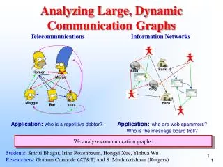
Outline • Defining a Dynamic Graph, and our objectives • A motivating example: Repetitive fraud in telecommunications • Our approach: representation and approximation of dynamic graphs • Revisiting Repetitive Fraud • Parameter setting and applications to other domains • Fraud revisited – applying our methods • Other applications, conclusions, further work Summary • Analyzing large dynamic graphs of transactional data is hard! • By storing and analyzing a massive graph as an indexed set of small local graphs, we have developed a generic framework for dynamic graph representation, which facilitates fast and accurate analysis.
Defining Dynamic Graphs Chris Corinna Daryl Anne Debby Jen Fred Zach John • Dynamic Graphs represent transactional data – • Credit card data • Web connectivity data • Web logs • Telecommunications network traffic • Online auction data Transactional data can be represented as a directed graph… Kathleen
Defining Dynamic Graphs • Dynamic Graphs • Nodes represent transactors • Edges are directed transactions • All edges have a time stamp • All edges have a weight (?) • May contain • Other attributes on nodes • Other attributes on edges
Analysis of dynamic graphs Why is it hard? • Scale • Often tens or hundreds of millions of nodes and edges • Doesn’t fit in main memory • Dynamic • Large numbers of nodes coming and going continuously • Accounting for temporal component of changing graphs is a challenge • Heterogeneous nodes • Superactive nodes dominate visualization and analysis • Zipf’s law holds: most users have few connections
Overview: Our Objectives • Define a representation for a dynamic graph • What is the graph at time t: Gt • How does one account for addition and attrition of nodes • Graphs can be used for • Global properties - learning about the graph properties • Clustering coefficient • Power law coefficient • Graph depth • Local represenation – learning about individual nodes in the graph • Entities – the local subgraph of a node of interest • Fraud signatures, anomaly (intrusion) detection, matching, etc. • Our Goal: Methods for entity based analysis in large dynamic graphs
A motivating example: Repetitive fraud in telecommunications
Motivating Example: Repetitive Fraud • Lots of people cant pay their bill, but they want phone service anyway:
Motivating Example: Repetitive Fraud How can we identify that it is the same person behind both accounts?
Motivating Example: Challenges 10 K/day 300K/month Connect pool T Restrict pool 5 K/day 150 K/month 45 billion comparisons • This is a problem of record linkage and graph matching, but because of obfuscation, we can only count on the graph matching! • But the problem is huge: • Q: How can we do efficient matching to put a dent in this problem? • A: Efficient representation of entities
Our graph is large 350M Telephone numbers (TNs) currently active on our Long Distance network, 300M calls/day Our graph is dynamic Motivating Example: Our data 4 Million TNs appear per week 4 Million TNs disappear per week
Motivating Example: Our data 95% = 171 Median = 34 Our graph is sparse: For one year of long distance data:
Our Approach to Dynamic Graphs • Definition • Representation • Approximation
Our Approach: Defining dynamic graphs • We could use: • We could use the union of all time periods: • We could use a moving average of the most recent time periods: • Q: for transactional data, what does the graph at time t (Gt)mean? - let gt be the collection of nodes and edges during the time period t Too narrow! Too broad! Too many!
Our Approach: Defining dynamic graphs We adopt an Exponentially Weighted Moving Average (EWMA): i.e. today’s graph is defined recursively as a convex combination of yesterday’s graph and today’s data Alternatively, this is: Through time, edge weights decay with decay rate q • Advantages: • recent data has most influence • only one most recent graph need be stored
Our Approach: Defining dynamic graphs Selecting q • closer to 1 • calls decay slower • more historical data included • smoother • q closer to 0 • faster decay • recent calls count more • more power to detect changes • less smooth q = 1/(1-n) means weight reduces to 1/e times its original weight in n days
Our Approach: Representation 2222222222 100.3 1111111111 90.1 3213232423 27.0 9098765453 11.3 8876457326 5.4 2122121212 3.0 9908989898 0.9 8887878787 0.1 • Since we are interested in entities, we represent the graph as a union of entity graphs • These entity graphs are the atomic units of analysis, a signature of the behavior of the node • As it turns out, storing hundreds of millions of small graphs is much more efficient than storing one massive graph. We use Hancock, a language developed at AT&T for signatures, which allows for easy indexed storage of • In short, we are approximating a hugh graph with many little graphs, which are easily accessible (via indexed storage) for analysis.
Our Approach: Representation 1111111111 92.1 2222222222 90.3 3213232423 24.3 9098765453 10.1 8876457326 4.9 2122121212 3.7 9991119999 0.5 3990898989 0.8 8887878787 0.09 Update the graph by updating all of the atomic units daily – so any time we access the data we have the most recent representation. Yesterday’s graph Today’s data Today’s graph 2222222222 100.3 1111111111 90.1 3213232423 27.0 9098765453 11.3 8876457326 5.4 2122121212 3.0 9908989898 0.9 8887878787 0.1 1111111111 20.0 2122121212 10.0 9991119999 5.0 + =
Our Approach: Approximation 1111111111 92.1 2222222222 90.3 3213232423 24.3 9098765453 10.1 8876457326 4.9 2122121212 3.7 9991119999 0.5 3990898989 0.8 8887878787 0.09 1111111111 92.1 2222222222 90.3 3213232423 24.3 9098765453 10.1 8876457326 4.9 2122121212 3.7 Other 1.4 = • We also implore two types of approximation of the graph, by pruning. • Local pruning of edges – designate a maximal in and out degree (k) for each node, and assign an overflow bin • Global pruning of edges – overall threshold (e) below which edges are removed from the graph • Removes stale edges • Reduces effect of supernodes
Our Approach: Approximation • Defending k • Most entities have the vast majority of their weight in a fraction of their nodes
Our Approach: Parameter Selection • We have now defined a representation of a dynamic graph by three parameters: • q - controls the decay of edges and edge weights • e - global pruning parameter • k – local pruning parameter • For a given application, we choose the parameters by optimizing predictive performance, selecting the parameters which optimize a loss function • Two loss functions we have used: • Weighted Dice • Hellinger Distance
Our Approach: Parameter Selection • Let A and B be two entities. • Weighted Dice: • Hellinger Distance: • For each value • Set e to be a low tolerance value • For a range of k, optimize q • Look at the plot to select parameters
Our Approach: Summary • This method allows us, for all 350 million phone numbers we see on the network to have an up-to-date representation of the entity associated with each number. These entities are stored in an indexed data base for easy storage and retrieval • Parameters are set to maximize the self-similarity of a node with itself through time, to allow us to match entities.
Fraud Revisited: Applying our methods • Fraudsters don’t get caught, so they go elsewhere • Can we find them, based on their calling patterns? • Intuition: fraudster may change network identity, but calling pattern will be similar • Find overlap in calling pattern between recent connected lines and lines shut down for fraud.
Fraud Revisited: Applying our methods 10 K/day 300K/month 5 K/day 150 K/month • Repetitive Fraud Process Connect pool T Restrict pool • Anchor on a few restrict dates in the pool • Compare to all connects in the connect pool • For all of those that have at least one overlap, collect more information
Fraud Revisited: Applying our methods TN-1 Connect TN-2 Restrict TN-3 TN-4 Connect TN-5 • For each potential matched pair • Calculate a matching score, based on the characteristics of the overlap: • Incorporate other information, including • Name, address • Payment history • Tenure
Fraud Revisited: Applying our methods • Results: • We identify 50-100 of these cases a day • 95% match rate • 85% block rate • Credited with saving AT&T $5M in reduced costs and uncollectables in 2002-2003 • By far the most reliable matching criteria is the entity based matching
Other applications, conclusions, further work • We have a representation of a dynamic graph which can be applied to any problem where entity modeling over time is of interest • Other fraud: GBA • Language models • Email • Web pages • Terrorism • Viral Marketing • Targeting • Understanding
Matching Algorithm • What cases will we present to the reps? • A combination of: • COI Overlap measures • At least two, and strength determined by uniqueness of overlap TNs • Name/address overlap • Edit distance no more than 50% of the longest name or address • $$ owed • Most interested in the ones that will generate the most $$ • 500-1000 cases a day become 100-150 that we present to the reps
Motivating Example: Repetitive Fraud • When we catch a fraudster, we rarely catch the person, we simply shut down the line • They will likely move on to another attempt at defrauding us, from a different network location • Idea: record linkage - network identity has changed, but network behavior is the same • We can use network behavior to indicate that the new line has the same “owner” as an old line
COI Signatures to COI • To construct a COI from a COI signature: • Often the signature contains things we don’t want: • Businesses • High weight nodes • Often the signature doesn’t contain things we do want: • Local calls • Other carrier calls • To combat this, create a COI by: • Recursively expanding the COI signature • Adding edges • Pruning edges here’s an example…
COI signature other me other
Extended COI other me other
Enhanced COI other me other
Pruned COI other me other
A likely case of the same fraudster showing up as a new number Pink nodes exist in both COI
Fraud Revisited: Applying our methods B Z A O Where: wao = weight of edge from a to o wob = weight of edge from o to b wo= sum weight of edges to o dao, dob are the graph distances from a and b to o • Calculate the “informative overlap” score: wob wao wo