Download

1 / 34
340 likes | 344 Views
This report provides an overview of regional price parities (RPPs) and their use in comparing price levels across different regions. It includes methodology, data sources, and results for state RPPs. The report also discusses the use of RPPs to adjust data for regional price differences.

E N D
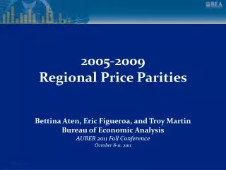
Regional Price Parities Bettina Aten, Eric Figueroa and Troy Martin rpp@bea.gov Bureau of Economic Analysis
OverviewSpatial vs Time-to-time Price Indexes • Multilateral Price indexes: • PPPs (purchasing power parities) in the international literature, with a choice of numeraire currency, such as Euro, or US Dollar • RPPs (regional price parities) within a country, same currency • Other types of Spatial Price indexes: • Bilateral • Cost of Living
Overview of BEA-BLS-Census Collaboration • Office of Prices and Living Conditions at the Bureau of Labor Statistics (BLS) • CPI prices • Expenditure weights • Poverty Statistics Branch, Housing and Household Economic Statistics (HHES) at the Census Bureau • American Community Survey • Housing survey
Overview of Data • Consumer Price Index (CPI) micro data on prices from BLS • 207 item strata, 38 urban areas (1 million observations / year) • Rents and Owners’ Equivalent Rents (34,000 observations / year) • Consumer Expenditure Survey (CE) weights data from BLS • 207 item-level weights x 38 urban areas • Plus 207 item-level weights x 4 rural areas • American Community Survey (ACS) from Census • 51 states, 363 metro areas, 3143 counties: Rent price levels • 5 year rolling average for all counties (10 million observations for 5 years)
Results: State RPPs • RPPs show percent difference in price levels: • Across regions • For one specified time period • Price level across all regions and expenditures equals 100 * Includes Washington, DC.
Results: State RPPs • RPPs show percent difference in price levels: • Average price level in Hawaii is 18.5% higher than the national average. 118.5 / 100 = 1.185 • Average price level of goods in Hawaii is 15.8% higher than in South Dakota. 106.3 / 91.8 = 1.158 * Includes Washington, DC.
Methodology • Estimation of Price levels and Expenditure Weights (annual BLS inputs) • Hedonic and shortcut regressions; separate rent and owner-occupied rent regressions for 38 BLS areas; • Multilateral price indexes for 207 items and 38 BLS areas • Allocation and Imputation (multiyear ACS and BEA inputs) • Allocation of price levels and weights to counties • Redistribution to match BEA’s Personal Consumption Expenditure weights at the national level • Imputation of Owner occupied rents using ACS and BLS housing data • Aggregation • Multilateral price indexes: annual for 51 states, three-year average for 363 metro areas, five-year average for countires.
Price levelsHedonic Regressions • Hedonic adjustment • Price quotes are controlled to characteristics provided by CPI-checklists. • Improves measurement of area coefficients • For all items in the Top 75 item strata by expenditure weight. • Covers about 85% of total expenditures • 700 unique regressions for 2005-2009
Multilateral Aggregation (3) Weighted CPD Notation and formulas follow Deaton & Dupriez (2009). P = price index, p = item price, s = budget share, q = notional quantity Subscript i = 1…N indicates items; j = 1…M indicates areas; c, d indicate areas c,d.
Multilateral Aggregation N = 207 item categoriesM = 38 BLS areas Notation and formulas follow Deaton & Dupriez (2009). P = price index, p = item price, q = notional quantity = (pq)/p Subscript I = 1…N indicates items; j = 1…M indicates areas; c, d also indicate areas.
RPPs by Expenditure Class and Type of County Rental costs are 1.6 times higher on average in Metro vs. Rural areas (106 / 67)
RPPs by Expenditure Class and Type of County Rural areas tend to have more inexpensive services relative to goods.
Using RPPs to Adjust Data Controls for differences in regional price levels: 54.6 / 31.2 = 1.75 Unadjusted PI is 75% higher in Hawaii than in South Dakota. After adjustment, PI is only 24% higher in Hawaii. 46.1 / 37.3 = 1.24 * Includes Washington, DC.
31 of these are self-representing PSUs (A PSUs) with population exceeding 1.5 million* * Anchorage, AK and Honolulu, HI are A PSUs with smaller populations.
Next are 4 sets of B PSUs; these smaller metropolitan areas have codes that begin with “X”.
Next largest set of areas are 3C PSUs (size class D). These nonmetropolitan urban areas have codes that begin with “D”.
Together, the A, B and C PSU’s make up the urban portion of the US.
Allocations • Assumptions: • Price levels of the counties within BLS areas equal the price level of the BLS area • Expenditure weights within areas proportional to income • Except for Rents: • Use actual ACS county level observations on Rent price levels and expenditures • Use BLS relationship between Rent price level and Owner-occupied price levels to impute Owner-occupied rent expenditures, by type of structure and number of bedrooms
ACS Rents • Close collaboration with the Poverty Statistics Branch of the Housing and Household Economic Statistics Division (HHES) of the Census Bureau to process the housing component of the ACS • American Community Survey ( multiyear rolling average for all counties in the U.S.) • About 3 million observations on rents in the housing survey • Hedonic regression for individual housing units • Dependent variable = log of gross rents ($) • Characteristics include number of bedrooms, type of unit (apartment, detached house, etc.), year built, total number of rooms, and the survey year (2005-2009) • Geographic coefficients by state (51 including DC), metro areas (366 as defined by OMB) and three groupings (metro, micro and rural) also OMB defined
Final Multilateral Aggregation • Five-year averages for BLS price levels • Food, Apparel, Education, Medical, Transport, Recreation, Housing (excluding Rents) and Other goods • Multiyear Rent and Owner-occupied rent levels: • Annual for States • Three-year for MSAs • Five-year for counties • One RPP for each state, metro area and type of county
5-Year Average RPPs by State Hawaii (118) Arizona, Florida, Rhode Island All U.S. = 100 South Dakota (84)
RPPs on the BEA website: www.bea.gov Research at BEA > Browse by Topic > Price Indexes
BEA Working Papers • 2005-2009 excel tables include these data: * As defined by the Office of Management and Budget
Future Development • RPPs by States, Metro and County Type for 2006-2010 • May 2012 • RPPs using Personal Consumption Expenditures (BEA concept) • Currently using Consumption Expenditure concept used at BLS • Differences in weights and coverage • Owner-Occupied Rent price levels and expenditures • Currently using Rents for both Renters and Owner-Occupied homes
Selected References • ACS estimates of geographic differences can be found at: http://www.census.gov/hhes/povmeas/publications/working.html • Deaton, Angus. “Price Indexes, Inequality, and the Measurement of World Poverty.” American Economic Review 2010, 100:1, 5-34. • Deaton, Angus and Olivier Dupriez. “Purchasing Power Parity Exchange Rates for the Global Poor.” http://princeton.edu/~deaton/downloads/Purchasing_power_parity_exchange_rates_for_global_poor_Nov11.pdf • Renwick, Trudi. “Alternative Geographic Adjustments of U.S. Poverty Thresholds: Impact on State Povery Rates.” U.S. Census Bureau 2009, http://www.census.gov/hhes/www/povmeas/papers/Geo-Adj-Pov-Thld8.pdf • Verbrugge, Randal and Thesia Garner. “Reconciling User Costs and Rental Equivalence: Evidence from the U.S. Consumer Expenditure Survey.” U.S. Bureau of Labor Statistics 2009, Working Papers 247.
Multilateral Aggregation (1) Gini-EKS Tornqvist Notation and formulas follow Deaton & Dupriez (2009). P = price index, p = item price, s = budget share, q = notional quantity Subscript i = 1…N indicates items; j = 1…M indicates areas; c, d indicate areas c,d.
Multilateral Aggregation (2) Gini-EKS Fisher Notation and formulas follow Deaton & Dupriez (2009). P = price index, p = item price, s = budget share, q = notional quantity Subscript i = 1…N indicates items; j = 1…M indicates areas; c, d indicate areas c,d.