ENEE759K/CMSC751: Parallel Algorithmics, Spring 2012 Time and Location MW 2:00-3:15. JMP 2202

1. ENEE759K/CMSC751: Parallel Algorithmics, Spring 2012 Time and Location • MW 2:00-3:15. JMP 2202 Instructor: Dr. U. Vishkin • E-mail: vishkin@umd.edu • Office hours: M 5:00-6:00 (by appointment) at AVW 2365 TA • James Edwards, jedward5@umd.edu Home Page • http://www.umiacs.umd.edu/users/vishkin/TEACHING/enee759k-s12.html Did you get my test email? Main way for course announcements

2. Course Goals Introduction to the theory of parallel algorithms Parallel algorithmic thinking obtaining good speed-ups over best serial algorithm. Class presentations & dry HW Study the theory of parallel algorithms; design & asymptotic analysis of parallel algorithms. Programming reduce to practice. Why? Hard speedups on real HW (XMT)  1. Improved understanding. 2. YOU can do it: (i) in course assignments. (ii) for most advanced algorithms studied. Examination: (still open) CS&E research questionWill the emerging ``Billion-transistor-per-chip'' era provide a way for building a truly general-purpose parallel computer system on-chip? Focus Single program completion time. (Throughput is important, but is a different challenge)

3. How to Think Algorithmically in Parallel? Uzi Vishkin

4. Commodity computer systems Chapter 1 19462003:Serial. 5KHz4GHz. Chapter 2 2004--: Parallel. #”cores”:~dy-2003 Apple 2004: 1 core 2008: 8 cores 2012: ?? cores Windows 7: scales to 256 cores… how to use the remaining 255? Is this the role of the OS? BIG NEWS Clock frequency growth: flat. If you want your program to run significantly faster … you’re going to have to parallelize it Parallelism: only game in town Since 1980: #Transistors/chip 29K~10sB! Bandwidth/Latency 300X [HP12] Programmer’s IQ? Flat.. 40 years of parallel computing The world is yet to see a successful general-purpose parallel computer: Easy to program & good speedups Intel Platform 2015, March05

5. 2 Paradigm Shifts • Serial to parallel: widely agreed • Within parallel: Imported from supercomputing “Decomposition-first” paradigm. Painful to program. Proposed paradigm Express only “what can be done in parallel”. Easy-to-program.

6. Abstractions in CS • Any particular word of an indefinitely large memory is immediately available • A uniprocessor is serving the task that the user is currently working on exclusively. (i) abstracts away a hierarchy of memories, each has greater capacity, but slower access time, than the preceding one. (ii) abstracts way: virtual file systems that can be implemented in local storage or a local or global network, the (whole) web, and other tasks that may be concurrently using the same computer system. These abstractions have improved productivity of programmers and other users, and contributed towards broadening participation in computing. • The proposed addition to this consensus is as follows. That an indefinitely large number of operations available for concurrent execution executes immediately.

7. The Pain of Parallel Programming Parallel programming is currently too difficult: To many users programming existing parallel computers is “as intimidating and time consuming as programming in assembly language” [NSF Blue-Ribbon Panel on Cyberinfrastructure]. AMD/Intel: “Need PhD in CS to program today’s multicores”. The real problem: Parallel architectures built using the following “methodology”: build-first figure-out-how-to-program-later. [J. Hennessy: “Many of the early ideas were motivated by observations of what was easy to implement in the hardware rather than what was easy to use”] Tribal lore, parallel programming profs, DARPA HPCS Development Time study (2004-2008): “Parallel algorithms and programming for parallelism is easy.What is difficult is the programming/tuningfor performance that comes after that.”

8. Who should produce the parallel code? Thanks: Prof. Barua Choices [state-of-the-art compiler research perspective] • Programmer only • Writing parallel code is tedious. • Good at ‘seeing parallelism’, esp. irregular parallelism. • But are bad at seeing locality and granularity considerations. • Have poor intuitions about compiler transformations. • Compiler only • Can see regular parallelism, but not irregular parallelism. • Great at doing compiler transformations to improve parallelism, granularity and locality.  Hybrid solution: Programmer specifies high-level parallelism, but little else. Compiler does the rest. Goals: • Ease of programming • Declarative programming (My) Broader questions Where will the algorithms come from? Is today’s HW good enough? This course relevant for all 3 questions

9. Welcome to today’s impasse/denial “All” vendors committed to multi-cores. Yet, their architecture and how to program them for single program completion time not clear/stable/robust  The software spiral (HW improvements  SW imp  HW imp) – growth engine for IT (A. Grove, Intel); Alas, now broken! SW vendors avoid investment in long-term SW development since may bet on the wrong horse. Impasse bad for business Diminished competition among HW vendors. Parallel programming education: Does CS&E degree mean: being trained for a 50yr career dominated by parallelism by programming yesterday’s serial computers? If no, why not same impasse? Can teach common denominator (grad, seniors, freshmen, HS)  the education enterprise has an actionable agenda!

10. But, what is this common denominator? Serial RAM Step: 1 op (memory/etc). PRAM (Parallel Random-Access Model) Step: many ops. Serial doctrine Natural (parallel) algorithm time = #ops time << #ops 1979- : THEORY figure out how to think algorithmically in parallel 1997- : PRAM-On-Chip@UMD: derive specs for architecture; design and build Note 2 issues: (i) parallel algorithmic thinking, (ii) specs first. What could I do in parallel at each step assuming unlimited hardware  . . # ops . . # ops . . .. .. .. .. time time

11. Flavor of parallelism Exchange Problem Replace A and B. Ex. A=2,B=5A=5,B=2. Serial Alg: X:=A;A:=B;B:=X. 3 Ops. 3 Steps. Space 1. Fewer steps (FS): X:=A B:=X Y:=B A:=Y 4 ops. 2 Steps. Space 2. Array Exchange Problem Given A[1..n] & B[1..n], replace A(i) and B(i), i=1..n. Serial Alg: For i=1 to n do X:=A(i);A(i):=B(i);B(i):=X /*serial replace 3n Ops. 3n Steps. Space 1. Par Alg1: For i=1 to n pardo X(i):=A(i);A(i):=B(i);B(i):=X(i) /*serial replace in parallel 3n Ops. 3 Steps. Space n. Par Alg2: For i=1 to n pardo X(i):=A(i) B(i):=X(i) Y(i):=B(i) A(i):=Y(i) /*FS in parallel 4n Ops. 2 Steps. Space 2n. Discussion Parallelism requires extra space (memory). Par Alg 1 clearly faster than Serial Alg. Is Par Alg 2 preferred to Par Alg 1?

12. Snapshot: XMT High-level language XMTC: Single-program multiple-data (SPMD) extension of standard C. Includes Spawn and PS - a multi-operand instruction. Short (not OS) threads. Cartoon Spawn creates threads; a thread progresses at its own speed and expires at its Join. Synchronization: only at the Joins. So, virtual threads avoid busy-waits by expiring. New: Independence of order semantics (IOS). Array Exchange. Pseudo-code for Par Alg1 Spawn(1,n){ X($):=A($);A($):=B($);B($):=X($) }

13. Example of Parallel algorithm Breadth-First-Search (BFS)

16. (i) “Concurrently” as in natural BFS: only change to serial algorithm (ii) Defies “decomposition”/”partition” Parallel complexity W = ~(|V| + |E|) T = ~d, the number of layers Average parallelism = ~W/T Mental effort 1. Sometimes easier than serial 2. Within common denominator of other parallel approaches. In fact, much easier

17. 1st example for denial [EduPar2011] 2011 NSF/IEEE-TCPP curriculum teach BFS using OpenMP Teaching experiment Joint F2010 UIUC/UMD class. 42 students Good news Easy coding (since no meaningful ‘decomposition’) Bad newsNone got speedup over serial on 8-proc SMP machine BFS alg was easy but .. no good: no speedups Speedups on 64-processor XMT 7x to 25x Fair to compare 64 processors to 8 since <1/4 of the silicon area Symptom of the bigger denial ‘Only problem Developers lack parallel programming skills’ Solution Education. False Teach then see that HW is the problem. Secret Nobody demands hard speedups from undergrads, but be quiet$$$ HotPAR10 performance results include BFS: XMT/GPU Speed-up same silicon area, highly parallel input: 5.4X Small HW configuration, large diameter: 109X wrt same GPU

18. Discussion of BFS results • Contrast with smartest people, Stanford’11, Nvidia’12 .. BFS on multi-cores/GPUs, again only if the diameter is small, improving on a SC’10 IBM/GaTech and 6 other recent papers, all 1st rate conferences. BFS is bread & butter. Call the Marines each time you need bread? Makes one wonderWhat is wrong with this field?! • ‘Decree’ Random graphs = ‘reality’. In the old days: Expander graphs taught in graph design. Planar graphs were real • Lots of parallelism  more HW design freedom. E.g., GPUs get decent speedup with lots of parallelism. But, not enough for general parallel algorithms. BFS (& max-flow): better speedups and easier programs on XMT

19. More Order-of-Magnitude Denial Examples 1 Performance ExampleParallelMax-Flow speedups vs best serial • [HeHo, IPDPS10] <= 2.5x using best of CUDA & CPU hybrid • [CarageaV, SPAA11] <= 108.3x using XMT (ShiloachV&GoldbergTarjan) Big effort beyond published algorithms vs normal theory-to-practice • Advantage by 43X Why max-flow example? • As advanced any irregular fine-grained parallel algorithms dared on any parallel architecture • - Horizons of a computer architecture cannot only be studied using elementary algorithms [Performance, efficiency and effectiveness of a car not tested only in low gear or limited road conditions] • Stress test for important architecture capabilities not often discussed: • Strong scaling : Increase #processors, not problem size • Rewarding even little amounts of algorithm parallelism with speedups

20. Ease of programmingEase of learning. Teachability [SIGCSE’10] • Freshman class. 11 non-CS students. Prog. assignments: merge-sort*, integer-sort* & sample-sort. • TJ Magnet HS (5th year). Teacher downloaded simulator, assignments, class notes, from XMT page. Self-taught. • Recommends Teach XMT first. Easiest to set up (simulator), program, analyze - predictable performance (as in serial). Not just embarrassingly parallel. Teaches also OpenMP, MPI, CUDA ** - HS & MS (some 10 yr old) from underrepresented groups by HS Math teacher • Benchmark Can any CS major program your manycore? for hard speedups? Avoiding it  denial & … state-of-the-art • Programmability necessary condition for success of a many core platform. Teachability necessary for that & a practical benchmark. • *In Nvidia + UC Berkeley IPDPS09 research paper! • **Also, keynote at CS4HS’09@CMU + interview with teacher More Order-of-Magnitude Denial Examples 2

21. Middle School Summer Camp Class, July’09 (20 of 22 students). Math HS Teacher D. Ellison, U. Indiana

22. Independent validation by DoD employeeIt all got started in CMSC751, spring 2010 Nathaniel Crowell. Parallel algorithms for graph problems, May 2011. MSc scholarly paper, CS@UMD. Not part of the XMT team http://www.cs.umd.edu/Grad/scholarlypapers/papers/NCrowell.pdf • Evaluated XMT for public domain problems of interest to DoD • Developed serial then XMT programs • Solved with minimal effort (MSc scholarly paper..) many problems. E.g., 4 SSCA2 kernels, Algebraic connectivity and Fiedler vector (Parallel Davidson Eigensolver) • Good speedups • No way where one could have done that on other parallel platforms so quickly • Reports: extra effort for producing parallel code was minimal Greater opportunity now New graph-theory library. Extra credit opportunity: biconnectivity prog. assignment.

23. “The U.S. Is Busy Building Supercomputers, but Needs Someone to Run Them”*, 12/2011 • ‘Low-end’ supercomputers $1-10M/unit • Supercomputing leaders Not enough programmers Comments 1. Fewer (total) programmers than many-cores 2. Prog. models of many-cores too similar to expect a difference 3. IMO denial. Just a symptom. The problem is the HW Space <~1TB main memory. If 1000-core HW, order-of-magnitude: • Lower Cost (~$10K/unit), • Easier programming • Greater speedups (performance) Research opportunity Anybody interested: Bioinformatics? ‘Watson technologies’? HTML5? Compiler… PhD each. * http://www.thedailybeast.com/articles/2011/12/28/the-u-s-is-busy-building-supercomputers-but-needs-someone-to-run-them.html

24. Need A general-purpose parallel computer framework [“successor to the Pentium for the multi-core era”] that: is easy to program; gives good performance with any amount of parallelism provided by the algorithm; namely, up- and down-scalability including backwards compatibility on serial code; supports application programming (VHDL/Verilog, OpenGL, MATLAB) and performance programming; and fits current chip technology and scales with it. (in particular: strong speed-ups for single-task completion time) Main Point of talk: PRAM-On-Chip@UMD is addressing (i)-(iv).

25. The macro technical pictureIt is all about (2nd class) levers Credit: Archimedes • Parallel algorithms. First principles. Alien culture: had to do from scratch. (No lever) • Levers: • 1. Input: Parallel algorithm. Output: Parallel architecture. • 2. Input: Parallel algorithms & architectures. Output: parallel programming

26. The PRAM Rollercoaster ride Late 1970’s Theory work began UP Won the battle of ideas on parallel algorithmic thinking. No silver or bronze! Model of choice in all theory/algorithms communities. 1988-90: Big chapters in standard algorithms textbooks. DOWN FCRC’93: “PRAM is not feasible”. [‘93+ despair no good alternative! Where vendors expect good enough alternatives to come from now?]; Device changed it all: UP Highlights: eXplicit-multi-threaded (XMT) FPGA-prototype computer (not simulator), SPAA’07,CF’08; 90nm ASIC tape-outs: int. network, HotI’07, XMT. # on-chip transistors How come? crash “course” on parallel computing How much processors-to-memories bandwidth? If enough: Ideal Programming Model (PRAM) If limited: Programming difficulties

27. The eXplicit MultiThreading (XMT) Easy-To-Program Parallel Computer www.umiacs.umd.edu/users/vishkin/XMT

28. The XMT Overall Design Challenge Spectrum of Explicit Multi-Threading (XMT) Framework Algorithms −− > architecture −− > implementation. XMT: strategic design point for fine-grained parallelism New elements are added only where needed Attributes Holistic: A variety of subtle problems across different domains must be addressed: Understand and address each at its correct level of abstraction

29. Not just talking Algorithms PRAM-On-Chip HW Prototypes 64-core, 75MHz FPGA of XMT (Explicit Multi-Threaded) architecture SPAA98..CF08 128-core intercon. networkIBM 90nm: 9mmX5mm, 400 MHz [HotI07]Fund work on asynch NOCS’10 FPGA designASIC IBM 90nm: 10mmX10mm PRAM parallel algorithmic theory. “Natural selection”. Latent, though not widespread, knowledgebase ICE/WorkDepth Conjecture SV82: The rest (full PRAM algorithm) just a matter of skill Lots of evidence that “work-depth” works. Used as framework in main PRAM algorithms texts: JaJa92, KKT01 programming & workflow Stable compiler. Architecture scales to 1000+ cores on-chip

30. Naming Contest for New Computer (2007) Paraleap chosen out of ~6000 submissions Single (hard working) person (X. Wen) completed synthesizable Verilog description AND the new FPGA-based XMT computer in slightly more than two years. No prior design experience. Attests to: basic simplicity of the XMT architecture  faster time to market, lower implementation cost.

31. Experience with High School Students, Fall’07 1-day parallel algorithms tutorial to 12 HS students. Some (2 10th graders) managed 8 programming assignments, including 5 of the 6 in the grad course. Only help: 1 office hour/week by undergrad TA. No school credit. Part of a computer club after 8 periods/day. One of these 10th graders: “I tried to work on parallel machines at school, but it was no fun: I had to program around their engineering. With XMT, I could focus on solving the problem that I had to solve.”

32. Software release Allows to use your own computer for programming on an XMT environment and experimenting with it, including: Cycle-accurate simulator of the XMT machine Compiler from XMTC to that machine Also provided, extensive material for teaching or self-studying parallelism, including Tutorial + manual for XMTC (150 pages) Classnotes on parallel algorithms (100 pages) Video recording of 9/15/07 HS tutorial (300 minutes) Next Major Objective Industry-grade chip and production quality compiler. Requires 10X in funding.

33. Current Participants Grad students: James Edwards, Beliz Saybasili, Alex Tzannes*. Recent grads: Aydin Balkan, George Caragea, Mike Horak, Fuat Keceli, Xingzhi Wen • Industry design experts (pro-bono). • Rajeev Barua, Compiler. Co-advisor X2. NSF grant. • Gang Qu, VLSI and Power. Co-advisor. • Steve Nowick, Columbia U., Asynch computing. Co-advisor. NSF team grant. • Ron Tzur, U. Colorado, K12 Education. Co-advisor. NSF seed funding K12:Montgomery Blair Magnet HS, MD, Thomas Jefferson HS, VA, Baltimore (inner city) Ingenuity Project Middle School 2009 Summer Camp, Montgomery County Public Schools • Marc Olano, UMBC, Computer graphics. Co-advisor. • Tali Moreshet, Swarthmore College, Power. Co-advisor. • Bernie Brooks, NIH. Co-Advisor. • Marty Peckerar, Microelectronics • Igor Smolyaninov, Electro-optics • Funding: NSF, NSA deployed XMT computer, NIH • Reinvention of Computing for Parallelism. 1st out of 49 for Maryland Research Center of Excellence (MRCE) by USM. Not yet funded. 17 members, including UMBC, UMBI, UMSOM. Mostly applications. * 1st place, ACM Student Research Competition, PACT, Oct 2011. Post-doc UIUC

34. Principled Objective of the Course Ideal: Present an untainted view of the only truly successful theory of parallel algorithms. Why is this easier said than done? Theory (3 dictionary definitions):  * A body of theorems presenting a concise systematic view of a subject. An unproved assumption: conjecture. FCRC’93: “PRAM infeasible” 2nd def not good enough “Success is not final, failure is not fatal: it is the courage to continue that counts” W. Churchill Feasibility proof status: programming & real hw that scales to cutting edge technology. Involves a real computer: CF’08PRAM is becoming feasible Achievable: Minimally tainted view. Also promotes * to: The principles of a science or an art.

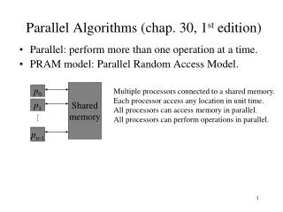
35. Parallel Random-Access Machine/Model PRAM: • n synchronous processors all having unit time access to a shared memory. • Each processor has also a local memory. • At each time unit, a processor can: • write into the shared memory (i.e., copy one of its local memory registers into • a shared memory cell), • 2. read into shared memory (i.e., copy a shared memory cell into one of its local • memory registers ), or • 3. do some computation with respect to its local memory.

36. pardo programming construct - for Pi , 1 ≤ i ≤ n pardo - A(i) := B(i) This means The following n operations are performed concurrently: processor P1 assigns B(1) into A(1), processor P2 assigns B(2) into A(2), …. Modeling read&write conflicts to the same shared memory location Most common are: - exclusive-read exclusive-write (EREW) PRAM: no simultaneous access by more than one processor to the same memory location for read or write purposes • concurrent-read exclusive-write (CREW) PRAM: concurrent access for reads but not for writes • concurrent-read concurrent-write (CRCW allows concurrent access for both reads and writes. We shall assume that in a concurrent-write model, an arbitrary processor among the processors attempting to write into a common memory location, succeeds. This is called the Arbitrary CRCW rule. There are two alternative CRCW rules: (i) Priority CRCW: the smallest numbered, among the processors attempting to write into a common memory location, actually succeeds. (ii) Common CRCW: allows concurrent writes only when all the processors attempting to write into a common memory location are trying to write the same value.

37. Example of a PRAM algorithm: The summation problem Input An array A = A(1) . . .A(n) of n numbers. The problem is to compute A(1) + . . . + A(n). The summation algorithm works in rounds. Each round: add, in parallel, pairs of elements: add each odd-numbered element and its successive even-numbered element. If n = 8, outcome of 1st round is: A(1) + A(2), A(3) + A(4), A(5) + A(6), A(7) + A(8) Outcome of 2nd round: A(1) + A(2) + A(3) + A(4), A(5) + A(6) + A(7) + A(8) and the outcome of 3rd (and last) round: A(1) + A(2) + A(3) + A(4) + A(5) + A(6) + A(7) + A(8) B – 2-dimensional array (whose entries are B(h,i), 0 ≤ h ≤ log n and 1 ≤ i ≤ n/2h) used to store all intermediate steps of the computation (base of logarithm: 2). For simplicity, assume n = 2k for some integer k. ALGORITHM 1 (Summation) 1. for Pi , 1 ≤ i ≤ n pardo 2. B(0, i) := A(i) 3. for h := 1 to log n do 4. if i ≤ n/2h 5. then B(h, i) := B(h − 1, 2i − 1) + B(h − 1, 2i) 6. else stay idle 7. for i = 1: output B(log n, 1); for i > 1: stay idle Algorithm 1 uses p = n processors. Line 2 takes one round, Line 3 defines a loop taking log n rounds Line 7 takes one round.

38. Summation on an n = 8 processor PRAM Again Algorithm 1 uses p = n processors. Line 2 takes one round, line 3 defines a loop taking log n rounds, and line 7 takes one round. Since each round takes constant time, Algorithm 1 runs in O(log n) time. [When you see O (“big Oh”), think “proportional to”.] So, an algorithm in the PRAM model is presented in terms of a sequence of parallel time units (or “rounds”, or “pulses”); we allow p instructions to be performed at each time unit, one per processor; this means that a time unit consists of a sequence of exactly p instructions to be performed concurrently. So, an algorithm in the PRAM model is presented in terms of a sequence of parallel time units (or “rounds”, or “pulses”); we allow p instructions to be performed at each time unit, one per processor; this means that a time unit consists of a sequence of exactly p instructions to be performed concurrently.

39. 2 drawbacks to PRAM mode: (i) Does not reveal how the algorithm will run on PRAMs with different number of processors; e.g., to what extent will more processors speed the computation, or fewer processors slow it? (ii) Fully specifying the allocation of instructions to processors requires a level of detail which might be unnecessary (a compiler may be able to extract from lesser detail) Work-Depth presentation of algorithms Alternative model and presentation mode. Work-Depth algorithms are also presented as a sequence of parallel time units (or “rounds”, or “pulses”); however, each time unit consists of a sequence of instructions to be performed concurrently; the sequence of instructions may include any number.

40. WD presentation of the summation example “Greedy-parallelism”: At each point in time, the (WD) summation algorithm seeks to break the problem into as many pair wise additions as possible, or, in other words, into the largest possible number of independent tasks that can performed concurrently. ALGORITHM 2 (WD-Summation) 1. for i , 1 ≤ i ≤ n pardo 2. B(0, i) := A(i) 3. for h := 1 to log n 4. for i , 1 ≤ i ≤ n/2h pardo 5. B(h, i) := B(h − 1, 2i − 1) + B(h − 1, 2i) 6. for i = 1 pardo output B(log n, 1) The 1st round of the algorithm (lines 1&2) has n operations. The 2nd round (lines 4&5 for h = 1) has n/2 operations. The 3rd round (lines 4&5 for h = 2) has n/4 operations. In general, the k-th round of the algorithm, 1 ≤ k ≤ log n + 1, has n/2k-1 operations and round log n +2 (line 6) has one more operation (use of a pardo instruction in line 6 is somewhat artificial). The total number of operations is 2n and the time is log n + 2. We will use this information in the corollary below. The next theorem demonstrates that the WD presentation mode does not suffer from the same drawbacks as the standard PRAM mode, and that every algorithm in the WD mode can be automatically translated into a PRAM algorithm.

41. The WD-presentation sufficiency Theorem Consider an algorithm in the WD mode that takes a total of x = x(n) elementary operations and d = d(n) time. The algorithm can be implemented by any p = p(n)-processor PRAM within O(x/p + d) time, using the same concurrent-write convention as in the WD presentation. [i.e., 5 theorems: EREW, CREW, Common/Arbitrary/Priority CRCW] Proof xi - # instructions at round i. [x1+x2+..+xd = x] p processors can simulate xiinstructions in ⌈xi/p⌉≤ xi/p + 1 time units. See next slide. Demonstration in Algorithm 2’ shows why you don’t want to leave this to a programmer. Formally: first reads, then writes. Theorem follows, since ⌈x1/p⌉+⌈x2/p⌉+..+⌈xd/p⌉≤ (x1/p +1)+..+(xd/p +1) ≤ x/p + d

42. Round-robin emulation of y concurrent instructions by p processors in ⌈y/p⌉ rounds. In each of the first ⌈y/p⌉ −1 rounds, p instructions are emulated for a total of z = p(⌈y/p⌉ − 1) instructions. In round ⌈y/p⌉, the remaining y − z instructions are emulated, each by a processor, while the remaining w − y processor stay idle, where w = p⌈y/p⌉

43. Corollary for summation example Algorithm 2 would run in O(n/p + log n) time on a p-processor PRAM. For p ≤ n/ log n, this implies O(n/p) time. Later called both optimal speedup & linear speedup For p ≥ n/ log n: O(log n) time. Since no concurrent reads or writes  p-processor EREW PRAM algorithm.

44. ALGORITHM 2’ (Summation on a p-processor PRAM) 1. for Pi , 1 ≤ i ≤ p pardo 2. for j := 1 to ⌈n/p⌉ − 1 do - B(0, i + (j − 1)p) := A(i + (j − 1)p) 3. for i , 1 ≤ i ≤ n − (⌈n/p⌉ − 1)p - B(0, i + (⌈n/p⌉ − 1)p) := A(i + (⌈n/p⌉ − 1)p) - for i , n − (⌈n/p⌉ − 1)p ≤ i ≤ p - stay idle 4. for h := 1 to log n 5. for j := 1 to ⌈n/(2hp)⌉ − 1 do (*an instruction j := 1 to 0 do means: - “do nothing”*) • B(h, i+(j −1)p) := B(h−1, 2(i+(j −1)p)−1) + B(h−1, 2(i+(j −1)p)) 6. for i , 1 ≤ i ≤ n − (⌈n/(2hp)⌉ − 1)p - B(h, i + (⌈n/(2hp)⌉ − 1)p) := B(h − 1, 2(i + (⌈n/(2hp)⌉ − 1)p) − 1) + - B(h − 1, 2(i + (⌈n/(2hp)⌉ − 1)p)) - for i , n − (⌈n/(2hp)⌉ − 1)p ≤ i ≤ p - stay idle • for i = 1 output B(log n, 1); for i > 1 stay idle Nothing more than plugging in the above proof. Main point of this slide: compare to Algorithm 2 and decide, which one you like better But is WD mode as easy as it gets? Hold on…Key question for this presentation

45. Measuring the performance of parallel algorithms A problem. Input size: n. A parallel algorithm in WD mode. Worst case time: T(n); work: W(n). 4 alternative ways to measure performance: 1. W(n) operations and T(n) time. 2. P(n) = W(n)/T(n) processors and T(n) time (on a PRAM). 3. W(n)/p time using any number of p ≤ W(n)/T(n) processors (on a PRAM). 4. W(n)/p + T(n) time using any number of p processors (on a PRAM). Exercise 1: The above four ways for measuring performance of a parallel algorithms form six pairs. Prove that the pairs are all asymptotically equivalent.

46. Goals for Designers of Parallel Algorithms Suppose 2 parallel algorithms for same problem: 1. W1(n) operations in T1(n) time. 2. W2(n) operations, T2(n) time. General guideline: algorithm 1 more efficient than algorithm 2 if W1(n) = o(W2(n)), regardless of T1(n) and T2(n); if W1(n) and W2(n) grow asymptotically the same, then algorithm 1 is considered more efficient if T1(n) = o(T2(n)). Good reasons for avoiding strict formal definition—only guidelines ExampleW1(n)=O(n),T1(n)=O(n); W2(n)=O(n log n),T2(n)=O(log n) Which algorithm is more efficient? Algorithm 1: less work. Algorithm 2: much faster. In this case, both algorithms are probably interesting. Imagine two users, each interested in different input sizes and in different target machines (different # processors). For one user Algorithm 1 faster. For second user Algorithm 2 faster. Known unresolved issues with asymptotic worst-case analysis.

47. Nicknaming speedups Suppose T(n) best possible worst case time upper bound on serial algorithm for an input of length n for some problem. (T(n) is serial time complexity for problem.) Let W(n) and Tpar(n) be work and time bounds of a parallel algorithm for same problem. The parallel algorithm is work-optimal, if W(n) grows asymptotically the same as T(n). A work-optimal parallel algorithm is work-time-optimal if its running time T(n) cannot be improved by another work-optimal algorithm. What if serial complexity of a problem is unknown? Still an accomplishment if T(n) is best known and W(n) matches it. Called linear speedup. Note: can change if serial improves. Recall main reasons for existence of parallel computing: - Can perform better than serial - (it is just a matter of time till) Serial cannot improve anymore

48. Default assumption regarding shared memory access resolution Since all conventions represent virtual models of real machines: strongest model whose implementation cost is “still not very high”, would be practical. Simulations results + UMD PRAM-On-Chip architecture • Arbitrary CRCW NC Theory Good serial algorithms: poly time. Good parallel algorithm: poly-log time, poly processors. Was much more dominant than what’s covered here in early 1980s. Fundamental insights. Limited practicality. In choosing abstractions: fine line between helpful and “defying gravity”

49. Technique: Balanced Binary Trees; Problem: Prefix-Sums Input: Array A[1..n] of elements. Associative binary operation, denoted ∗, defined on the set: a ∗ (b ∗ c) = (a ∗ b) ∗ c. (∗ pronounced “star”; often “sum”: addition, a common example.) The n prefix-sums of array A are: A(1) A(1) ∗ A(2) .. A(1) ∗ A(2) ∗ .. ∗ A(i) .. A(1) ∗ A(2) ∗ .. ∗ A(n) Prefix-sums is perhaps the most heavily used routine in parallel algorithms.

50. ALGORITHM 1 (Prefix-sums) 1. for i , 1 ≤ i ≤ n pardo - B(0, i) := A(i) 2. for h := 1 to log n 3. for i , 1 ≤ i ≤ n/2h pardo - B(h, i) := B(h − 1, 2i − 1) ∗ B(h − 1, 2i) 4. for h := log n to 0 5. for i even, 1 ≤ i ≤ n/2h pardo - C(h, i) := C(h + 1, i/2) 6. for i = 1 pardo - C(h, 1) := B(h, 1) 7. for i odd, 3 ≤ i ≤ n/2h pardo - C(h, i) := C(h + 1, (i − 1)/2) ∗ B(h, i) 8. for i , 1 ≤ i ≤ n pardo - Output C(0, i) } Summation (as before) } C(h,i) – prefix-sum of rightmost leaf of [h,i]