Download
1 / 31
310 likes | 318 Views
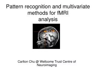
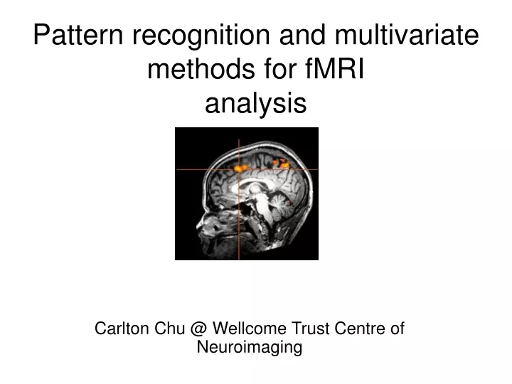
Pattern recognition and multivariate methods for fMRI analysis. Carlton Chu @ Wellcome Trust Centre of Neuroimaging. Time. Intensity time series of a particular voxel Y. Mass univariate approach. =. Parameter beta. Error. Design matrix X. Covariance. Voxel 1 (intensity).

E N D
Pattern recognition and multivariate methods for fMRIanalysis Carlton Chu @ Wellcome Trust Centre of Neuroimaging
Time Intensity time series of a particular voxel Y Mass univariate approach = Parameter beta Error Design matrix X
Covariance Voxel 1 (intensity) Voxel 2 (intensity)
Principle Components Minor variance component Major variance component
Principle Components Analysis (PCA) is the new rotated matrix
Weight (w) Prediction model (decoding) ACTIVITY Stimuli or design paradigm =
Learning to Predict • The main achievement of science is predictive accuracy • Theories (models) describe probabilistic relationships among empirically observed data. • Good models predict unobserved data, from other data. • Interpolative prediction • Extrapolative prediction • Science advances by replacing old models with those with greater predictive accuracy. • Bayesian model selection indicates predictive accuracy.
Learning the pattern • The goal is to create a mapping y= f(x) between the input features and the targets (classes for classification, values for regression) Supervised Learning Algorithm (Optimize function of x and training error) Training data {x,y} Features {x} Predicted {y} Traget {y} Training error Error function
? ? ? ? Training and Classifying Group 2 Group 1
? ? ? ? Classifying Group 2 Group 1 y=f(aTx+b)
Support Vector Classifier a is a weighted linear combination of the support vectors Support Vector Support Vector Support Vector
Validation Supervised Learning Algorithm Training Training set {x,y} Collected data {x,y} Supervised Learning Algorithm After training Predicted {y} {x} Testing set {x,y} Validation Error {y}
n- fold Validation Data collected {x,y}, divide into n subsets Use 1 subset for testing Use n-1 subsets for training • Repeat n times until every subset is used as a testing set • In the case where n= total number of samples, then it is called leave one out cross validation
3 way splits Data collected {x,y}, split into 3 sets Use 1 subset for validating the parameters Leave 1 subset for testing Use n-2 subsets for training • Split into training, validating and testing set. Use the validation set to adjust the model parameters. • We normally leave one set out, then apply cross-validation on the remaining n-1 set to tune the parameters.
Weight Volume Subject13 Face Subject14 Velocity Subject1 Instruction
Single volumes classification Weight vector Face task x Location task Location task (x) and Face task (o) Janaina Mourão-Miranda,
Conclusion • Pattern recognition methods open a new window toward fMRI • analysis • Predictability and the predictive validity give the measure of pattern evidence and generalizability • Bayesian model comparison also arises different measure of pattern evidence • Useful pattern can be utilized such as lie detection or clinical diagnosis
MVB Decoding Practical Ollie Hulme 02/04/08
Experimental Design: Designing experiments suitable for MVB Preparation: Prerequisite processing steps for MVB Guide: Button-by-button step through guide MVB Decoding Practical: Contents Ollie Hulme 02/04/08
What types of design allow me to do an MVB analysis? MVB constitutes a decoding model that uses exactly the same design matrices of experimental variables X and neuronal responses Y as used in conventional analyses. X-data: Anything you would put in the design matrix. standard onset regressors (zeroth order) parametric regressors (n-order) Block vs. event related regressors Usually these encode the perceptual or behavioural states but can include physiological recordings (GSR, eyemovements etc), diagnostic information (medical, personality) and even activity of other parts of the brain (presumably a prinicipal component from an ROI) Y-data: Any data you would normally be interested Functional or Structural (e.g. grey matter metrics) MVB Decoding Practical: Experimental Design Ollie Hulme 02/04/08
contrast < < 50 100 SPM{F } 2,335 150 200 < 250 SPMresults: 300 Height threshold F = 7.052 350 2 4 6 Design matrix Statistics: search volume: 16.0mm sphere at [48,-63,0] set-level cluster-level voxel-level mm mm mm p c p k p p p F ( Z ) p corrected E uncorrected FWE-corr FDR-corr º uncorrected 0.006 4 39 0.000 0.000 40.66 Inf 0.000 39 -72 0 0.000 0.000 40.09 Inf 0.000 42 -75 -3 3 0.002 0.000 13.35 4.55 0.000 39 -63 -12 1 0.124 0.003 8.67 3.52 0.000 51 -66 -3 1 0.436 0.010 7.36 3.18 0.001 48 -63 0 table shows 16 local maxima more than 4.0mm apart 0 0 Height threshold: F = 7.05, p = 0.001 (0.513) {p<0.001 (unc.)} 0.1 0.2 0.3 0.4 0.5 Degrees of freedom = [2.0, 335.0] 0.6 0.7 0.8 0.9 1 Extent threshold: k = 0 voxels, p = 1.000 (0.513) FWHM = 7.5 7.4 7.1 mm mm mm; 2.5 2.5 2.4 {voxels}; Expected voxels per cluster, <k> = 1.212 Volume: 15741; 583 voxels; 43.3 resels Expected number of clusters, <c> = 0.72 Voxel size: 3.0 3.0 3.0 mm mm mm; (resel = 14.69 voxels) Expected false discovery rate, <= 0.01 Simply estimate your regression model and calculate a contrast for your target variables. MVB Decoding Practical: Preconditions for MVB Centre the cursor on your ROI Note: Anecdotally for very large design matrices, 1000 volumes x 300 regressors MVB can crash. Ollie Hulme 02/04/08
Specify search volume according to anatomical hypotheses. Pragmatically, memory capacity constrains size of search. Anecdotally: with 2G RAM 20mm radius too large, 10mm fine. (Also likely to vary as a function of the design matrix you are applying it too) MVB Decoding Practical: Button pressing Specify spatial model to compute Ollie Hulme 02/04/08
MVB is not just for establishing the statistical dependency between the target variable and the neural data. It is designed to compare different models of that mapping. Different models specifying different priors on the mapping. Key concept is sparsity. MVB Decoding Practical: Spatial models Grandmother cells Mass action sparse distributed Spatial: models sparse representations over anatomy, analogous to functional segregation. Few voxels have large variance, most have small Smooth: models sparse representations that are spatially coherent over anatomy Singular: models distributed representations that are sparse in pattern space, meaning only a small number of distributed patterns expressed at any time Support: models distributed representations that are not sparse in pattern space, meaning a large number of distributed patterns is expressed. sparse distributed Ollie Hulme 02/04/08
distribution of weights 600 500 400 frequency 300 200 100 0 -0.03 -0.02 -0.01 0 0.01 0.02 voxel-weight MVB Decoding Practical: Results Note sparsity- few voxels with high weights most with zero weight. Heavy tails indicate anatomical sparsity. Posterior probabilities (that weights are non-zero) of 16 most significant voxels spaced >4mm apart. ROI must be large enough. posterior probability map showing which voxels contribute to the decoding for the model of interest- Plot of observed and predicted target over scans Observed vs predicted. If perfect should be straight diagonal Ollie Hulme 02/04/08
MVB Decoding Practical: Model comparison within area Select all models of interest Repeat for each of the 4 models of interest (saving under different names) A standard threshold is 3 meaning that the model is 20 times (exp(3)) more likely than another- in this case the null model Bayes factor spatial singular support smooth null Ollie Hulme 02/04/08
MVB Decoding Practical: Model comparison across areas b Ollie Hulme 02/04/08