Download
1 / 40
400 likes | 496 Views
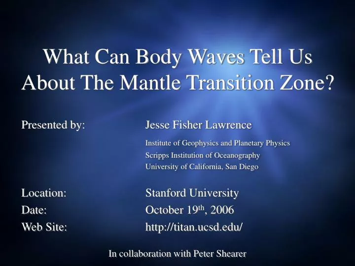
What Can Body Waves Tell Us About The Mantle Transition Zone?. Presented by: Jesse Fisher Lawrence Institute of Geophysics and Planetary Physics Scripps Institution of Oceanography University of California, San Diego Location: Stanford University Date: October 19 th , 2006

E N D
What Can Body Waves Tell Us About The Mantle Transition Zone? Presented by: Jesse Fisher Lawrence Institute of Geophysics and Planetary Physics Scripps Institution of Oceanography University of California, San Diego Location: Stanford University Date: October 19th, 2006 Web Site: http://titan.ucsd.edu/ In collaboration with Peter Shearer
General Structure of the Earth: [Dziewonski and Anderson, 1981: PEPI] From http://garnero.ucsd.edu/
Why Study the Transition Zone? Phase changes associated with the discontinuities inhibit mantle flow to some extent. • How much depends on the density contrasts, which can vary from place to place. • The transition zone can also change as a result of convection.
Phase Transformations: • While most velocity & density jumps are near 410 & 660 km depth, the actual depth can vary depending on temperature. • In seismology we can measure waves that reflect off of these discontinuities. [e.g., Bina & Helffrich, 1994]
Receiver Functions: • P-to-S converted waves (Pds) : • Recorded 30-90 from earthquakes. • P-waves are recorded on the vertical component of a 3-component seismometer. • P & P-to-S converted waves are recorded on the radial horizontal component. [After Ammon, 1991: BSSA]
Receiver Functions: Vertical Record: dZ(t)=sZ(t)*fZ(t)*lZ(t)*iZ(t)*nZ(t) Radial Record: dR(t)=sR(t)*fR(t)*lR(t)*iR(t)*nR(t) • The receiver function is the vertical record deconvolved from the radial component. rf(t) =dR(t)*-1dZ(t) or rf(t) =lR(t)*-1lZ(t)+noise instrument source s i far field f l local n = noise
Receiver Functions: Spectral Division: or In practice this is:
Actual Receiver Functions: • Stacked Receiver functions isolate P660s & P410s well. • 3000 receiver functions can be calculated & stacked in ~10 minutes. • Little interference from other waves like PP and PcP. • 3317 traces added to this stack. [Lawrence & Shearer, 2006: JGR]
Look at 1D or 3D variations: [Lawrence & Shearer, 2006: JGR]
Unaligned SH waves Aligned SH waves 1 minute S410S S660S SS-Precursors: • Our understanding of the transition zone was revolutionized by work on SS-Precursors in the 1990’s. • Stack all available long-period records on the peak amplitude of the SS wave, • Group by distance, • Coherent signal constructively builds, • Incoherent signal destructively interferes. ScSScS [After Flanagan & Shearer 1998: JGR]
SS-Precursors: • Wave stripping: • S410S, S520S, S660S • The 520-km discontinuity, while week, is a robust global feature. • There is structure below the 660-km discontinuity. Sub-660 gradient [Shearer 1996: JGR]
PP PP-Precursors: • There is a strong P410P. • There is evidence of a P520P. • But where is P660P? • Is there no P660P? • Or are other waves interfering with it? • [Estabrook & Kind, 1996: Science] [Lawrence & Shearer, in press: G3]
Interference PdP Vertical Horizontal PP-Precursors: An Alternate Look [Lawrence & Shearer, in press G3]
PP-Precursors: 1D Stack • About 5-6 times the signal-to-noise ratio of the 2D stacks because there are 20-40 times more waves in each stack. • P660P and P520P do appear. • The radial and vertical stacks are very similar! P410P P660P? P520P? [Lawrence & Shearer, in press: G3]
Topside Ppdp Reflections: • Pp660p is weaker than Pp410p, but it is much stronger than P660P. • So why is the P660P so weak? • What is different about the 660? 660 [Lawrence & Shearer, in press: G3]
Receiver Functions: • While P410s & P660s are strong, where is P520s? • If anything, P520s has a negative impulse. • Why is the 520 different from the 410 and 660? [Lawrence & Shearer, in press: G3]
Modeling Method: • A linear inversion is problematic when fitting just one type of data. • We use the Niching Genetic Algorithm. • Solve for changes in: P-velocity: VP - 0-10% S-velocity: VS - 0-10% density: - 0-10% Interface Depth: z - 30 km Interface Thickness: H - 30 km • Synthetic calculations with generalized ray theory using a priori pulse & heterogeneity constraints. [Lawrence & Shearer, in press: G3]
Modeling Each Waveform: [Lawrence & Shearer, in press: G3]
The Most Optimal Model: [Lawrence & Shearer, in press: G3]
Comparing Models: • No 520-km discontinuity. • 660-km discontinuity depth is deeper. • There are a lot of assumptions that go into PREF (both seismic & mineral physics). • More similar than AK135 & PREM. • PREF (blue) is a suite of seismic models calculated from mineral physics properties of a pyrolitic composition mantle. [Camarano et al., 2005]
Big Picture Results: • Previously studies, lacking observations of a positive P520s pulse wrongly concluded that the absence of the 520-km discontinuity. • While the 660 likely impedes convection (to some extent), this effect is less as a gradient rather than a discontinuity. • The 410 is a lot like we thought it was. • The 520 is a discontinuity in density and VP, not VS. • The 660 is much less significant discontinuity, and more of a gradient. • If the interfaces have some finite thickness, then the 410 is ~3X thicker than the 660.
Transition Zone Thickness & Topography: • Topography of the 410 & 660 are anti-correlated • Average thickness 241 km. • Topography: 20 km [Flanagan & Shearer, 1998: JGR]
Models agree at long wavelengths: G&D02 • Degree-6 there is good agreement • But fine structures are harder to get. G&D02 [Gu & Dziewonski, 2002: JGR]
SS-Precursors v. Receiver Functions? • Chevrot et al., [1999]: • Average Thickness: ~252 km • Thickness Variation: 15 km • Low correlation with SS-precursor studies.
Receiver Functions: • Receiver function stacks for 118 stations • Mean thickness: 247 km. • Median thickness: 246 km. • Strong P410s & P660s • Most lack a P520s [Lawrence & Shearer, 2006: JGR]
Correcting Biases: • Bias 1: P & Pds actually follow slightly different paths through the Earth: • While Chevrot et al., [1999] accounted for this during stacking, they did not correct for this when calculating depth. • They simply corrected to a particular distance. • 2-4 km overestimation in Chevrot et al., [1999]. [Lawrence & Shearer, 2006: JGR]
SdS Pds SdS Correcting Biases: • Bias 2: Stations are predominantly on continents, not oceans, but the Earth is ~70% ocean. • When we look at the long wavelength (harmonic degrees l < 6) the Pds is very similar to SdS. • Average Thickness: 242 km • Thickness variation: ± 20 km. • Correlation at R2=0.5 [Lawrence & Shearer, 2006: JGR]
Higher Resolution: • Current stacking method requires large bin sizes. • Short wavelength is smoothed over • Amplitudes are less than they should be
[e.g. Dahlen, 2005: GJI] SS-Precursor Sensitivity Kernels:
[e.g. Dahlen, 2005: GJI] Discretization: • With larger blocks the pattern gets smeared out. • Less X-shaped. • More circular.
Adaptive Stacking: • SdS has a very small amplitude (often below the noise). • Stack > 100 traces to increase signal to noise: • Provides more reliable travel time. • I also stack the sensitivity kernels. • I then invert the stacked travel times and stacked sensitivity kernels for the true structure.
Sensitivity of a Stack: • The second problem: for a stable inversion, we must have lots of data. • Stack many times with different geometries • 100-1000 waveforms per stack • Bootstrap method (25 X) ensures stack stability • Stack with variable sized bins dt: SdS-SdSAK135 travel time residual Kij: Sensitivity of jth wave to topography in the ith block. zi: topography of the ithnode ~60,000 stacks 2X10⁸ non-zero Kji values.
Inversion: Transition Zone Thickness rk10 Stacks: • Similar but different. • Larger amplitude shorter wavelength features. • Some anomalies moved or disappeared. • Others appeared or strengthened. Inverted Structure:
Transition Zone Thickness Input: Reproduction: Test the Model (1): • Given our model (zi) and sensitivity (Kji), can we reproduce our stacks? Yes!
Transition Zone Thickness Input: Reproduction: Test the Model (2): • Given a checkerboard pattern (zi) and the sensitivity (Kji), can we reproduce the checkerboard from theoretical stacks? Yes!
What does this model show? 200 km • Slabs? • Expected from plate motion & tomography. 200 km 200 km 1000 km 250 km 250 km [Lithgow-Bertelloni & Richards, 1998: R. Geophys.]
What does this model show? • Slabs? • Expected from plate motion & tomography. • Hotspots? • From tomography & convection modeling. 200 km 200 km 250 km 250 km
Conclusions: • Our views of the transition zone are still in flux. • Even the average structure is taking on shape, which can be used to infer the mineral physics, geodynamic, and geochemical environment. • By improving upon old techniques, we gain insight into the nature of the transition zone. • Constraining the scale of transition zone thickness anomalies is crucial for understanding understanding how the transition zone interacts with slabs and plumes. • Thin slabs equate to through-going anomalies. • Broad anomalies equate to stagnant anomalies.