Download
1 / 56
560 likes | 714 Views
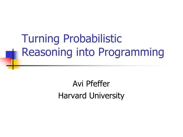
Turning Probabilistic Reasoning into Programming. Avi Pfeffer Harvard University. Uncertainty. Uncertainty is ubiquitous Partial information Noisy sensors Non-deterministic actions Exogenous events Reasoning under uncertainty is a central challenge for building intelligent systems.

E N D
Turning Probabilistic Reasoning into Programming Avi Pfeffer Harvard University
Uncertainty • Uncertainty is ubiquitous • Partial information • Noisy sensors • Non-deterministic actions • Exogenous events • Reasoning under uncertainty is a central challenge for building intelligent systems
Probability • Probability provides a mathematically sound basis for dealing with uncertainty • Combined with utilities, provides a basis for decision-making under uncertainty
Probabilistic Reasoning • Representation: creating a probabilistic model of the world • Inference: conditioning the model on observations and computing probabilities of interest • Learning: estimating the model from training data
The Challenge • How do we build probabilistic models of large, complex systems that are • easy to construct and understand • support efficient inference • can be learned from data
(The Programming Challenge) • How do we build programs for interesting problems that are • easy to construct and maintain • do the right thing • run efficiently
Lots of Representations • Plethora of existing models • Bayesian networks, hidden Markov models, stochastic context free grammars, etc. • Lots of new models • Object-oriented Bayesian networks, probabilistic relational models, etc.
Goal • A probabilistic representation language that • captures many existing models • allows many new models • provides programming-language like solutions to building and maintaining models
IBAL • A high-level “probabilistic programming” language for representing • Probabilistic models • Decision problems • Bayesian learning • Implemented and publicly available
Outline • Motivation • The IBAL Language • Inference Goals • Probabilistic Inference Algorithm • Lessons Learned
Stochastic Experiments • A programming language expression describes a process that generates a value • An IBAL expression describes a process that stochastically generates a value • Meaning of expression is probability distribution over generated value • Evaluating an expression = computing the probability distribution
Constants Variables Conditionals Stochastic Choice x = ‘hello y = x z = if x==‘bye ffthen 1 else 2 w = dist [ 0.4: ’hello, 0.6: ’world ] Simple expressions
Functions fair ( ) = dist [0.5 : ‘heads, 0.5 : ‘tails] x = fair ( ) y = fair ( ) • x and y are independent tosses of a ftfair coin
Higher-order Functions fair ( ) = dist [0.5 : ‘heads, 0.5 : ‘tails] biased ( ) = dist [0.9 : ‘heads, 0.1 : ‘tails] pick ( ) = dist [0.5 : fair, 0.5 : biased] coin = pick ( ) x = coin ( ) y = coin ( ) • x and y are conditionally independent ffgiven coin
Data Structures and Types • IBAL provides a rich type system • tuples and records • algebraic data types • IBAL is strongly typed • automatic ML-style type inference
D P(U| S, D) S s d 0.9 0.1 Diligent Smart s d 0.3 0.7 s d 0.6 0.4 Good Test Taker 0.01 0.99 s d Understands Exam Grade HW Grade Bayesian Networks nodes = domain variables edges = direct causal influence Network structure encodes conditional independencies: I(HW-Grade,Smart | Understands)
D S G U E H BNs in IBAL smart = flip 0.8 diligent = flip 0.4 understands = case <smart,diligent> of # <true,true> : flip 0.9 # <true,false> : flip 0.6 …
H1 H2 Ht-1 Ht O1 O2 Ot-1 Ot First-Order HMMs Initial distribution P(H1) Transition model P(Hi|Hi-1) Observation model P(Oi|Hi) What if hidden state is arbitrary data structure?
HMMs in IBAL init : () -> state trans : state -> state obs : state -> obsrv sequence(current) = { state = current observation = obs(state) future = sequence(trans(state)) } hmm() = sequence(init())
SCFGs S -> AB (0.6) S -> BA (0.4) A -> a (0.7) A -> AA (0.3) B -> b (0.8) B -> BB (0.2) • Non-terminals are data generating functions
SCFGs in IBAL append(x,y) = ifnull(x) then y else cons (first(x), append (rest(x),y) production(x,y) = append(x(),y()) terminal(x) = cons(x,nil) s() = dist[0.6:production(a,b), 0.4:production(b,a)] a() = dist[0.7:terminal(‘a),…
Actor Movie Gender Actor Genre Movie Chaplin Mod T. … … Appearance Actor Movie Role-Type Chaplin Mod T. … … Probabilistic Relational Models Role-Type Actor.Gender, Movie.Genre
PRMs in IBAL movie( ) = { genre = dist ... } actor( ) = { gender = dist ... } appearance(a,m) = { role_type = case (a.gender,m.genre) of (male,western) : dist ... } mod_times = movie() chaplin = actor() a1 = appearance(chaplin, mod_times)
Other IBAL Features • Observations can be inserted into programs • condition probability distribution over values • Probabilities in programs can be learnable parameters, with Bayesian priors • Utilities can be associated with different outcomes • Decision variables can be specified • influence diagrams, MDPs
Outline • Motivation • The IBAL Language • Inference Goals • Probabilistic Inference Algorithm • Lessons Learned
Goals • Generalize many standard frameworks for inference • e.g. Bayes nets, HMMs, probabilistic CFGs • Support parameter estimation • Support decision making • Take advantage of language structure • Avoid unnecessary computation
Diligent Smart Good Test Taker Understands Exam Grade HW Grade Desideratum #1: Exploit Independence • Use Bayes net-like inference algorithm
Desideratum #2: Exploit Low-Level Structure • Causal independence (noisy-or) x = f() y = g() z = x & flip(0.9) | y & flip(0.8)
Desideratum #2: Exploit Low-Level Structure • Context-specific independence x = f() y = g() z = case <x,y> of <false,false> : flip 0.4 <false,true> : flip 0.6 <true> : flip 0.7
Desideratum #3: Exploit Object Structure • Complex domain often consists of weakly interacting objects • Objects share a small interface • Objects are conditionally independent given interface Student 1 Student 2 Course Difficulty
Desideratum #4: Exploit Repetition • Domain often consists of many of the same kinds of objects • Can inference be shared between them? f() = complex x1 = f() x2 = f() … x100 = f()
Desideratum #5: Use the Query • Only evaluate required parts of model • Can allow finite computation on infinite model f() = f() x = let y = f() in true • A query on x does not require f • Lazy evaluation is required • Particularly important for probabilistic languages, e.g. stochastic grammars
Desideratum #6 Use Support • The support of a variable is the set of values it can take with positive probability • Knowing support of subexpressions can simplify computation f() = f() x = false y = if x then f() else true
Desideratum #7 Use Evidence • Evidence can restrict the possible values of a variable • It can be used like support to simplify computation f() = f() x = flip 0.6 y = if x then f() else true observe x = false
Outline • Motivation • The IBAL Language • Inference Goals • Probabilistic Inference Algorithm • Lessons Learned
Two-Phase Inference • Phase 1: decide what computations need to be performed • Phase 2: perform the computations
Natural Division of Labor • Responsibilities of phase 1: • utilizing query, support and evidence • taking advantage of repetition • Responsibilities of phase 2: • exploiting conditional independence, low-level structure and inter-object structure
Phase 1 IBAL Program Computation graph
Computation Graph • Nodes are subexpressions • Edge from X to Y means “Y needs to be computed in order to compute X” • Graph, not tree • different expressions may share subexpressions • memoization used to make sure each subexpression occurs once in graph
Construction of Computation Graph • Propagate evidence throughout program • Compute support for each node
Evidence Propagation • Backwards and forwards let x = <a:flip 0.4, b:1> in observe x.a = true in if x.a then ‘a else ‘b
Construction of Computation Graph • Propagate evidence throughout program • Compute support for each node • this is an evaluator for a non-deterministic programming language • lazy evaluation • memoization
Gotcha! • Laziness and memoization don’t go together • Memoization: when a function is called, look up arguments in cache • But with lazy evaluation, arguments are not evaluated before function call!
Lazy Memoization • Speculatively evaluate function without evaluating arguments • When argument is found to be needed • abort function evaluation • store in cache that argument is needed • evaluate the argument • speculatively evaluate function again • When function evaluates successfully • cache mapping from evaluated arguments to result
Need x Need y ‘a Lazy Memoization let f(x,y,z) = if x then y else z in f(true,’a,’b) f(_,_,_) f(true,_,_) f(true,’a,_)
Microfactors Solution P(Outcome=true)=0.6 Phase 2 Computation Graph
X Y Value False False 0 False True 1 True - 1 Microfactors • Representation of function from variables to reals • E.g. is the indicator function of XvY • More compact than complete tables • Can represent low-level structure
Producing Microfactors Goal: Translate an IBAL program into a set of microfactors F and a set of variables X such that the P(Output) = • Similar to Bayes net • Can solve by variable elimination • exploits independence
Producing Microfactors • Accomplished by recursive descent on computation graph • Use production rules to translate each expression type into microfactors • Introduce temporary variables where necessary
e1 e2 e3 X=False X=True e2 e3 X e1 X=True X=True X=False X=True 1 1 Producing Microfactors if e1then e2else e3