Download

1 / 52
520 likes | 592 Views
The Analysis and Forecast of Chinese Population. Instructor : 王凯波. Group Members: 李文华 2009210538 杨丽丹 2009210561 宋 芹 2009210568 杨春晖 2009220200. OUTLINE. PART 1:Introduction (Background, Objective, Terminology )

E N D
The Analysis and Forecast of Chinese Population Instructor: 王凯波 Group Members: 李文华 2009210538 杨丽丹 2009210561 宋 芹 2009210568 杨春晖 2009220200 IE @Applied Statistics, Group Report
OUTLINE PART 1:Introduction (Background, Objective, Terminology ) PART 2:Descriptive Analysis PART 3:Hypothesis Test of Male-Female Birth Rate (Descriptive date, Exploratory date , Cause analysis) PART 4:Fertility Comparison (Descriptive date , Exploratory date , Cause analysis) PART 5:Analysis of Ratio (Descriptive date , Exploratory date , Cause analysis) PART 6:Analysis of Dead Rate (Descriptive date , Exploratory date , Cause analysis) PART 7:Time Series Analysis of Total Population Size (Trend analysis, Model based analysis) PART 8: Conclusion
INTRODUCTION--Background • Before 1950 China had demographic characteristics of a pre-modern society with high dead rates and high fertility rates. This situation produced certain stability in population size or, at least, leads to a slow increase. • After the foundation of The People’s Republic of China in 1949, China entered its demographic transition: first dead rates began to fall rapidly and second, fertility remained for many years at about an average of six children per woman. As a result of this China experienced rapid population growth due to the high number of children born, a sharp decline of baby dead rate.
INTRODUCTION-China Population Today Now China has a population over 1.3 billion (2007), that is nearly 1/5 the world population. Most of the population are in the east (94%), which are more developed, and enjoying a relatively lower dead rate, and a lower baby dead rate
INTRODUCTION--Objective Our report would like to apply the statistics method with substantial evidence data got from CHINA POPULATION STATISTICS YEARBOOK (1995-2006) , and proceed the research and the analysis on the male-female birth rate, fertility rate and dead rate among different area (city, town, village), and different years, to have a trend analysis and prediction on the total China population.
INTRODUCTION--Terminology • City, Town & Village城市,乡镇,农村: City and Town in China is administratively defined as statutory cities and statutory towns judging from the population, economic, public finance and Infrastructure four aspects. Village is referred to the areas other than cities and towns. • Birth Rate (or crude birth rate) 出生率:The number of live births per 1,000 population in a given year. Not to be confused with the growth rate. • Death Rate (or crude death rate) 死亡率:The number of deaths per 1,000 population in a given year. • Sex Ratio出生人口性别比:The number of males per 100 females in a population. • Fertility Rate生育率:The number of live births per 1,000 women ages 15-44 or 15-49 years in a given year. ----Definition from Administrative Office of the State Council&Population Reference Bureau, USA
OUTLINE PART 1:Introduction (Background, Objective, Terminology ) PART 2:Descriptive Analysis PART 3:Hypothesis Test of Male-Female Birth Rate (Descriptive date, Exploratory date , Cause analysis) PART 4:Fertility Comparison (Descriptive date , Exploratory date , Cause analysis) PART 5:Analysis of Ratio (Descriptive date , Exploratory date , Cause analysis) PART 6:Analysis of Dead Rate (Descriptive date , Exploratory date , Cause analysis) PART 7:Time Series Analysis of Total Population Size (Trend analysis, Model based analysis) PART 8: Conclusion
DESCRIPTIVE ANALYSIS-Variables • Population size of China: • Fertility rate:(生育率) ‰ (1994-2005) • Male-female birth rate:F:100 (1994-2005) • Male (female) ratio of a certain age: % • the percentage of the male number of total male population. • Death rate: ‰
DESCRIPTIVE ANALYSIS-Data Sheet The data were collected from internet ,such as CHINA POPULATION STATISTICS YEARBOOK (1995-2006) (中国人口统计年鉴) etc.
DESCRIPTIVE ANALYSIS-Population size Observation: Continuous increase since 1962 Increase rate decrease last 20 years
DESCRIPTIVE ANALYSIS- Fertility rate Observation The age distribution of fertility is different. The birth peak for village comes earlier than city. And for all ages the village has higher birth rate.
DESCRIPTIVE ANALYSIS- Male/female rate of newborn Observation Jumping town data and stationary city and village data All exceed the rational range (102to 107)
DESCRIPTIVE ANALYSIS- Male-Female rate & death rate(2005) • Does there are any gender choice? • Does female lives longer?
OUTLINE PART 1:Introduction (Background, Objective, Terminology ) PART 2:Descriptive Analysis PART 3:Hypothesis Test of Male-Female Birth Rate (Descriptive date, Exploratory date , Cause analysis) PART 4:Fertility Comparison (Descriptive date , Exploratory date , Cause analysis) PART 5:Analysis of Ratio (Descriptive date , Exploratory date , Cause analysis) PART 6:Analysis of Dead Rate (Descriptive date , Exploratory date , Cause analysis) PART 7:Time Series Analysis of Total Population Size (Trend analysis, Model based analysis) PART 8: Conclusion
Male-Female Birth Rate--Data • Data selection: mainly survey and observation • 10 variables • 27,000 data points • Data process • integrate original data(15 forms) into one form • recalculate them to get new data • select data points to build a new sample e.g. fertility rate , death rate
Population Balance: Male-Female Birth Rate • (year:1994 -2005. type: city, town, village. 36 data points.) • One-way ANOVA: Male-female birth rate versus type (city, town and village) Main basis of population balance, of great importance. Number of baby boys when 100 baby girls:
Population Balance: Male-Female Birth Rate Conclusions and cause analysis: Three types own significant difference of gender balances and choices. P-value = 0.000<0.05 Boy preference: village (highest) town city (lowest) • Viewpoint that Man is superior to woman • The farm work and lifestyle • Education • Medical technique (helps sharpen the gender choice)
OUTLINE PART 1:Introduction (Background, Objective, Terminology ) PART 2:Descriptive Analysis PART 3:Hypothesis Test of Male-Female Birth Rate (Descriptive date, Exploratory date , Cause analysis) PART 4:Fertility Comparison (Descriptive date , Exploratory date , Cause analysis) PART 5:Analysis of Ratio (Descriptive date , Exploratory date , Cause analysis) PART 6:Analysis of Dead Rate (Descriptive date , Exploratory date , Cause analysis) PART 7:Time Series Analysis of Total Population Size (Trend analysis, Model based analysis) PART 8: Conclusion
Population replacement: Fertility rate • Main basis of population balance, of great importance. • number of babies per 1000 women from age 15-49: (year:1994 -2005. type: city, town, village. 2520 original points.)
Both significant! type difference: village> town> city year difference: negative trend Population replacement: Fertility rate • Two-way ANOVA: • Fertility rate versus type (city, town and village), year • Intersection of type and year • Conclusions and cause analysis: • It proves that one-child policy in our country works a lot. • Small rise and fall around 2003 result from the very epidemic SARS around 2003,which reduced the contact and pregnant chances.
Population replacement: Fertility rate Data process year(2001-2005), age( with highest fertility), type (city, town and village) Build up a new sample "fertility peak” • Scatter plot of fertility peak Fertility peak (highest fertility age) versus type, year • The age peak is around 24 • Fertility peak decreases • (city changes most. village most stable) • The village peak is the highest
OUTLINE PART 1:Introduction (Background, Objective, Terminology ) PART 2:Descriptive Analysis PART 3:Hypothesis Test of Male-Female Birth Rate (Descriptive date, Exploratory date , Cause analysis) PART 4:Fertility Comparison (Descriptive date , Exploratory date , Cause analysis) PART 5:Analysis of Ratio (Descriptive date , Exploratory date , Cause analysis) PART 6:Analysis of Dead Rate (Descriptive date , Exploratory date , Cause analysis) PART 7:Time Series Analysis of Total Population Size (Trend analysis, Model based analysis) PART 8: Conclusion
ANALYSIS of RATIO Step 1: Data collection Take city male ratio for example City male ratio=
ANALYSIS of RATIO Step 2: Descriptive date analysis In city, both male and female ratios are near 0.5. But the difference between male ratio and female ratio is getting larger and larger from town to village. Basically, there are more male than female in society. That is the reason why it is hard for many young men to find “Mrs. Right”.
ANALYSIS of RATIO Step 3 Exploratory date analysis
ANALYSIS of RATIO Step 3 Exploratory date analysis • Conclusion: • In city, male ratio is equal to female ratio. But it is larger than female ratio in town and village. • The difference between male ratio and female ratio is getting larger and larger from city to village.
ANALYSIS of RATIO Step 4 Cause analysis Reason 1 Reason 2 • City people • Just have one kid • Higher education • Higher pressures in life • Dink family • Town and village people • More than one kid • value the male child only And this phenomenon in village is more serious than that in town, so the difference between male ratio and female ratio in village is larger than that in town.
OUTLINE PART 1:Introduction (Background, Objective, Terminology ) PART 2:Descriptive Analysis PART 3:Hypothesis Test of Male-Female Birth Rate (Descriptive date, Exploratory date , Cause analysis) PART 4:Fertility Comparison (Descriptive date , Exploratory date , Cause analysis) PART 5:Analysis of Ratio (Descriptive date , Exploratory date , Cause analysis) PART 6:Analysis of Dead Rate (Descriptive date , Exploratory date , Cause analysis) PART 7:Time Series Analysis of Total Population Size (Trend analysis, Model based analysis) PART 8: Conclusion
ANALYSIS of DEAD RATE Step 1: Data collection Take city male dead rate for example City male dead rate ratio=
ANALYSIS of DEAD RATE Step 2: Descriptive date analysis Observation: male dead rate is higher than female’s. And there is another conclusion that the dead rate is increasing from city to village
ANALYSIS of DEAD RATE Step 3 Exploratory date analysis
ANALYSIS of DEAD RATE Step 3 Exploratory date analysis • Conclusion: • Male dead rate is higher than female dead rate • Dead rate is increasing from city to village
ANALYSIS of DEAD RATE Step 4 Cause analysis It is increasing from city to village 1:Male dead rate is higher • City • Higher education • Better living standard • Better medical care • Better work condition • reason • Male just have one X chromosome • Main labor force in society • Bad habit: smoking drinking • Accident, crime generally speaking, city better than town and village; and town is a little better than village.
OUTLINE PART 1:Introduction (Background, Objective, Terminology ) PART 2:Descriptive Analysis PART 3:Hypothesis Test of Male-Female Birth Rate (Descriptive date, Exploratory date , Cause analysis) PART 4:Fertility Comparison (Descriptive date , Exploratory date , Cause analysis) PART 5:Analysis of Ratio (Descriptive date , Exploratory date , Cause analysis) PART 6:Analysis of Dead Rate (Descriptive date , Exploratory date , Cause analysis) PART 7:Time Series Analysis of Total Population Size (Trend analysis, Model based analysis) PART 8: Conclusion
TOTAL POPULATION SIZE PREDICT-Guideline • The analysis here is based on the population data since the foundation of China, and based on 58 year’s population data we could do trend analysis and prediction in qualitative or quantitative analysis. • Trend analysis • Linear, exponential, quadratic and S-curve • Deviation analysis • ARIMA • Stationary • Model determination based on ACF/PACF • Prediction and deviation analysis
TOTAL POPULATION SIZE PREDICT- Trend object Continuous increase and a odd decrease point were observed in annually collected population data. From the Figure, we see the increase rate declined in last 20 years. China’s population has reached 132,129*104(2007) , we still face the serious population problem and also aging population problem too.
TOTAL POPULATION SIZE PREDICT- Result of trend analysis • Linear, exponential, quadratic and S-curve models were used to analysis the increase features. Parameters estimation is based on OLS methods. • 4 results were evaluated in 3 elementary indexes as MAD, MAPE, MSE. The result tells us that S-curve models fits China’s increase sharply then slowly reality.
TOTAL POPULATION SIZE PREDICT-Evaluation of 4 models Trends analysis’s use is to predict future. So we focus on the most recent regression deviation to evaluate these four models. That means we only take the deviation from 2000~2007.
TOTAL POPULATION SIZE PREDICT-ARIMA Description • ARIMA is developed by Box and Jenkins in 1970s, and it is a famous model in time serious analysis combined auto regression, moving average and also difference operation to treat unstationary time series data. • ARIMA(p,d,q), is determined in 3 step: • Stationary transfer • Model determination • Parameters estimation
TOTAL POPULATION SIZE PREDICT-Stationary Test A stationary time series data means the mean of the series does not change with time shift, and standard deviation could be limited in a range. Obvious increase trend was observed, so difference operation is needed to transfer the unstationary series into stationary one. But what is the difference order? “Augmented Dickey-Fuller , ADF” test is used in Matlab to test whether the series has a unit root.
TOTAL POPULATION SIZE PREDICT- One order difference solution P-value is smaller than 0.05, so we reject the null hypothesis. The series does not have unit root. It passes the AFD test and then come into the model determination part.
TOTAL POPULATION SIZE PREDICT- One order difference solution After determine the difference order of d=1, the ARIMA model turns into ARMA model. Model determination is based on ACF & PACF. ACF has a heavy tail and PACF is bobtail, then it is AR(1) model. So based on Box- Jenkins ARIMA(1,1,0)
TOTAL POPULATION SIZE PREDICT- One order difference solution • Residual check shows a odd points of “1961”. It is far from the normality line. What shall we do? • Transfer? • Cut the series? • We cut this series and take only 1962~2007.
TOTAL POPULATION SIZE PREDICT- Two order difference solution • AFD test? Decision vector H shows the 1962-2007 part is not a stationary series any more. And observation shows a decrease trend. So higher order difference is needed.
TOTAL POPULATION SIZE PREDICT- Two order difference solution • ARMA is of p=3, q=1 based on Box-Jenkins method • SS = 1114603, MS = 27865.
TOTAL POPULATION SIZE PREDICT- Two order difference solution ARIMA Model: C1 Final Estimates of Parameters Type Coef SE Coef T P AR 1 0.9138 0.0714 12.88 0.000 Constant 124.68 31.32 3.37 0.002 Mean 1313.7 390.3 Number of observations: 46 Residuals: SS = 1773508 (backforecasts excluded) MS = 40307 DF = 44 Population increase can be estimated by above function to get future value based on historical ones.
TOTAL POPULATION-Prediction and Deviation Analysis (2000-2007) Future increase and it 95% CI could be predicted, then the total population could be get respectably. MAPE dropped nearly 91%, MSD 99% and MAD 91%.
OUTLINE PART 1:Introduction (Background, Objective, Terminology ) PART 2:Descriptive Analysis PART 3:Hypothesis Test of Male-Female Birth Rate (Descriptive date, Exploratory date , Cause analysis) PART 4:Fertility Comparison (Descriptive date , Exploratory date , Cause analysis) PART 5:Analysis of Ratio (Descriptive date , Exploratory date , Cause analysis) PART 6:Analysis of Dead Rate (Descriptive date , Exploratory date , Cause analysis) PART 7:Time Series Analysis of Total Population Size (Trend analysis, Model based analysis) PART 8: Conclusion