Download
1 / 82
830 likes | 989 Views
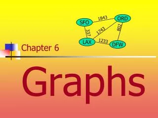
1843. ORD. SFO. 802. 1743. 337. 1233. LAX. DFW. Chapter 6 Graphs. Outline and Reading. Graphs ( § 6.1) Definition Applications Terminology Properties ADT Data structures for graphs ( § 6.2) Edge list structure Adjacency list structure Adjacency matrix structure.

E N D
1843 ORD SFO 802 1743 337 1233 LAX DFW Chapter 6Graphs
Outline and Reading • Graphs (§6.1) • Definition • Applications • Terminology • Properties • ADT • Data structures for graphs (§6.2) • Edge list structure • Adjacency list structure • Adjacency matrix structure
“To find the way out of a labyrinth there is only one means. At every new junction, never seen before, the path we have taken will be marked with three signs. If … you see that the junction has already been visited, you will make only one mark on the path you have taken. If all the apertures have already been marked, then you must retrace your steps. But if one or two apertures of the junction are still without signs, you will choose any one, making two signs on it. Proceeding through an aperture that bears only one sign, you will make two more, so that now the aperture bears three. All the parts of the labyrinth must have been visited if, arriving at a junction, you never take a passage with three signs, unless none of the other passages is now without signs.” --Ancient Arabic text
Graph Traversals • How do you find your way out of a maze, given a large supply of pennies? • Graph traversals • Depth-first search • Breadth-first search • Other applications: Boggle™, tic-tac-toe, path finding, theorem proving, motion planning, AI, …
A graph is a pair (V, E), where V is a set of nodes, called vertices E is a collection of pairs of vertices, called edges Vertices and edges are positions and store elements Example: A vertex represents an airport and stores the three-letter airport code An edge represents a flight route between two airports and stores the mileage of the route 849 PVD 1843 ORD 142 SFO 802 LGA 1743 337 1387 HNL 2555 1099 1233 LAX 1120 DFW MIA Graph
Edge Types • Directed edge • ordered pair of vertices (u,v) • first vertex u is the origin • second vertex v is the destination • e.g., a flight • Undirected edge • unordered pair of vertices (u,v) • e.g., a flight route • Directed graph • all the edges are directed • e.g., route network • Undirected graph • all the edges are undirected • e.g., flight network flight AA 1206 ORD PVD 849 miles ORD PVD
Applications • Electronic circuits • Printed circuit board • Integrated circuit • Transportation networks • Highway network • Flight network • Computer networks • Local area network • Internet • Web • Databases • Entity-relationship diagram
V a b h j U d X Z c e i W g f Y Terminology • End vertices (or endpoints) of an edge • U and V are the endpoints of a • Edges incident on a vertex • a, d, and b are incident on V • Adjacent vertices • U and V are adjacent • Degree of a vertex • X has degree 5 • Parallel edges • h and i are parallel edges • Self-loop • j is a self-loop
Terminology (cont.) • Path • sequence of alternating vertices and edges • begins with a vertex • ends with a vertex • each edge is preceded and followed by its endpoints • Simple path • path such that all its vertices and edges are distinct • Examples • P1=(V,b,X,h,Z) is a simple path • P2=(U,c,W,e,X,g,Y,f,W,d,V) is a path that is not simple V b a P1 d U X Z P2 h c e W g f Y
Terminology (cont.) • Cycle • circular sequence of alternating vertices and edges • each edge is preceded and followed by its endpoints • Simple cycle • cycle such that all its vertices and edges are distinct • Examples • C1=(V,b,X,g,Y,f,W,c,U,a,) is a simple cycle • C2=(U,c,W,e,X,g,Y,f,W,d,V,a,) is a cycle that is not simple V a b d U X Z C2 h e C1 c W g f Y
Notation n number of vertices m number of edges deg(v)degree of vertex v Property 1 Sv deg(v)= 2m Proof: each edge is counted twice Property 2 In an undirected graph with no self-loops and no multiple edges m n (n -1)/2 Proof: each vertex has degree at most (n -1) What is the bound for a directed graph? Properties Example • n = 4 • m = 6 • deg(v)= 3
Representing a Graph Two different drawings of the same graph are shown. • What data structure to represent this graph?
Adjacency Matrix A B C D E F G H I J K L M A 1 1 0 0 1 1 0 0 0 0 0 0 B 0 0 0 0 0 0 0 0 0 0 0 C 0 0 0 0 0 0 0 0 0 0 D 1 1 0 0 0 0 0 0 0 E 1 1 0 0 0 0 0 0 F 0 0 0 0 0 0 0 G 0 0 0 0 0 0 H 1 0 0 0 0 I 0 0 0 0 J 1 1 1 K 0 0 L 1 M Space required for a graph with v vertices, e edges? Q(v2) Time to tell if there is an edge from v1 to v2? Q(1)
Adjacency List A: F -> B -> C -> G B: A C: A D: E -> F E: D -> F -> G F: D -> E G: A -> E H: I I: H J: K -> L -> M K: J L: M -> J M: J -> L Space required for a graph with v vertices, e edges? Q(v+e) Time to tell if there is an edge from v1 to v2? Q(v)
Vertices and edges are positions store elements Accessor methods aVertex() incidentEdges(v) endVertices(e) isDirected(e) origin(e) destination(e) opposite(v, e) areAdjacent(v, w) Update methods insertVertex(o) insertEdge(v, w, o) insertDirectedEdge(v, w, o) removeVertex(v) removeEdge(e) Generic methods numVertices() numEdges() vertices() edges() Main Methods of the Graph ADT
A B D E C Depth-First Search
Outline and Reading • Definitions (§6.1) • Subgraph • Connectivity • Spanning trees and forests • Depth-first search (§6.3.1) • Algorithm • Example • Properties • Analysis • Applications of DFS (§6.5) • Path finding • Cycle finding
Subgraph Spanning subgraph Subgraphs • A subgraph S of a graph G is a graph such that • The vertices of S are a subset of the vertices of G • The edges of S are a subset of the edges of G • A spanning subgraph of G is a subgraph that contains all the vertices of G
A graph is connected if there is a path between every pair of vertices A connected component of a graph G is a maximal connected subgraph of G Connectivity Connected graph Non connected graph with two connected components
Trees and Forests • A (free) tree is an undirected graph T such that • T is connected • T has no cycles This definition of tree is different from the one of a rooted tree • A forest is an undirected graph without cycles • The connected components of a forest are trees Tree Forest
Spanning Trees and Forests • A spanning tree of a connected graph is a spanning subgraph that is a tree • A spanning tree is not unique unless the graph is a tree • Spanning trees have applications to the design of communication networks • A spanning forest of a graph is a spanning subgraph that is a forest Graph Spanning tree
Depth-first Search Main idea: keep traveling to a new, unvisited node until you you get stuck. Then backtrack as far as necessary and try a new path.
Depth-first search (DFS) is a general technique for traversing a graph A DFS traversal of a graph G Visits all the vertices and edges of G Determines whether G is connected Computes the connected components of G Computes a spanning forest of G DFS on a graph with n vertices and m edges takes O(n + m ) time DFS can be further extended to solve other graph problems Find and report a path between two given vertices Find a cycle in the graph Depth-first search is to graphs what Euler tour is to binary trees Depth-First Search
DFS Algorithm • The algorithm uses a mechanism for setting and getting “labels” of vertices and edges AlgorithmDFS(G, v) Inputgraph G and a start vertex v of G Outputlabeling of the edges of G in the connected component of v as discovery edges and back edges setLabel(v, VISITED) for all e G.incidentEdges(v) ifgetLabel(e) = UNEXPLORED w opposite(v,e) if getLabel(w) = UNEXPLORED setLabel(e, DISCOVERY) DFS(G, w) else setLabel(e, BACK) AlgorithmDFS(G) Inputgraph G Outputlabeling of the edges of G as discovery edges and back edges for all u G.vertices() setLabel(u, UNEXPLORED) for all e G.edges() setLabel(e, UNEXPLORED) for all v G.vertices() ifgetLabel(v) = UNEXPLORED DFS(G, v)
A A B D E B D E C C Example unexplored vertex A visited vertex A unexplored edge discovery edge backedge A B D E C
Example (cont.) A A B D E B D E C C A A B D E B D E C C
Non-recursive DFS • How can you implement DFS non-recursively? • Use a stack • For unconnected graphs, restart at unvisited nodes • Runtime? • O(n+m) AlgorithmDFS(G, v) Inputgraph G and a start vertex v of G Outputtraversal of the vertices of G in the connected component of v Stack S S.push(v) while S is not empty v S.pop() setLabel(v, VISITED) for each edge (v,w) out of v if w is UNEXPLORED, S.push(w)
DFS and Maze Traversal • The DFS algorithm is similar to a classic strategy for exploring a maze • We mark each intersection, corner and dead end (vertex) visited • We mark each corridor (edge) traversed • We keep track of the path back to the entrance (start vertex) by means of a rope (recursion stack)
Property 1 DFS(G, v) visits all the vertices and edges in the connected component of v Property 2 The discovery edges labeled by DFS(G, v) form a spanning tree of the connected component of v Properties of DFS A B D E C
Setting/getting a vertex/edge label takes O(1) time Each vertex is labeled twice once as UNEXPLORED once as VISITED Each edge is labeled twice once as UNEXPLORED once as DISCOVERY or BACK Method incidentEdges is called once for each vertex DFS runs in O(n + m) time provided the graph is represented by the adjacency list structure Recall that Sv deg(v)= 2m Analysis of DFS
Applications of DFS • How can you find a set of plane flights to get to your destination from your airport? • How can you tell if you can fly to all destinations from your airport? • How can you find a maximal set of plane flights that can be cancelled while still making it possible to get from any city to any other? • If computers have multiple network connections, how can you prevent routing storms?
Path Finding • How to find a path between vertices u and z? • Call DFS(G, u) with u as the start vertex • We use a stack S to keep track of the path between the start vertex and the current vertex • As soon as destination vertex z is encountered, we return the path as the contents of the stack AlgorithmpathDFS(G, v, z) setLabel(v, VISITED) S.push(v) if v= z return S.elements() for all e G.incidentEdges(v) ifgetLabel(e) = UNEXPLORED w opposite(v,e) if getLabel(w) = UNEXPLORED setLabel(e, DISCOVERY) S.push(e) pathDFS(G, w, z) S.pop(e) else setLabel(e, BACK) S.pop(v)
Cycle Finding • How to find a cycle in a graph? • We use a stack S to keep track of the path between the start vertex and the current vertex • When a back edge (v, w) is encountered, return the cycle as the portion of the stack from the top to w AlgorithmcycleDFS(G, v, z) setLabel(v, VISITED) S.push(v) for all e G.incidentEdges(v) ifgetLabel(e) = UNEXPLORED w opposite(v,e) S.push(e) if getLabel(w) = UNEXPLORED setLabel(e, DISCOVERY) pathDFS(G, w, z) S.pop(e) else T new empty stack repeat o S.pop() T.push(o) until o= w return T.elements() S.pop(v)
L0 A L1 B C D L2 E F Breadth-First Search
Outline and Reading • Breadth-first search (§6.3.3) • Algorithm • Example • Properties • Analysis • Applications • DFS vs. BFS (§6.3.3) • Comparison of applications • Comparison of edge labels
Breadth-first search (BFS) is a general technique for traversing a graph A BFS traversal of a graph G Visits all the vertices and edges of G Determines whether G is connected Computes the connected components of G Computes a spanning forest of G BFS on a graph with n vertices and m edges takes O(n + m ) time BFS can be further extended to solve other graph problems Find and report a path with the minimum number of edges between two given vertices Find a simple cycle, if there is one Breadth-First Search
BFS Algorithm • The algorithm uses a mechanism for setting and getting “labels” of vertices and edges AlgorithmBFS(G, s) L0new empty sequence L0.insertLast(s) setLabel(s, VISITED) i 0 while Li.isEmpty() Li +1new empty sequence for all v Li.elements() for all e G.incidentEdges(v) ifgetLabel(e) = UNEXPLORED w opposite(v,e) if getLabel(w) = UNEXPLORED setLabel(e, DISCOVERY) setLabel(w, VISITED) Li +1.insertLast(w) else setLabel(e, CROSS) i i +1 AlgorithmBFS(G) Inputgraph G Outputlabeling of the edges and partition of the vertices of G for all u G.vertices() setLabel(u, UNEXPLORED) for all e G.edges() setLabel(e, UNEXPLORED) for all v G.vertices() ifgetLabel(v) = UNEXPLORED BFS(G, v)
L0 A L1 B C D E F Example unexplored vertex A visited vertex A unexplored edge discovery edge crossedge L0 L0 A A L1 L1 B C D B C D E F E F
L0 L0 A A L1 L1 B C D B C D L2 E F E F L0 L0 A A L1 L1 B C D B C D L2 L2 E F E F Example (cont.)
L0 L0 A A L1 L1 B C D B C D L2 L2 E F E F Example (cont.) L0 A L1 B C D L2 E F
Notation Gs: connected component of s Property 1 BFS(G, s) visits all the vertices and edges of Gs Property 2 The discovery edges labeled by BFS(G, s) form a spanning tree Ts of Gs Property 3 For each vertex v in Li The path of Ts from s to v has i edges Every path from s to v in Gshas at least i edges Properties A B C D E F L0 A L1 B C D L2 E F
Setting/getting a vertex/edge label takes O(1) time Each vertex is labeled twice once as UNEXPLORED once as VISITED Each edge is labeled twice once as UNEXPLORED once as DISCOVERY or CROSS Each vertex is inserted once into a sequence Li Method incidentEdges is called once for each vertex BFS runs in O(n + m) time provided the graph is represented by the adjacency list structure Recall that Sv deg(v)= 2m Analysis
Applications • Using the template method pattern, we can specialize the BFS traversal of a graph Gto solve the following problems in O(n + m) time • Compute the connected components of G • Compute a spanning forest of G • Find a simple cycle in G, or report that G is a forest • Given two vertices of G, find a path in G between them with the minimum number of edges, or report that no such path exists
L0 A L1 B C D L2 E F DFS vs. BFS A B C D E F DFS BFS
Back edge(v,w) w is an ancestor of v in the tree of discovery edges Cross edge(v,w) w is in the same level as v or in the next level in the tree of discovery edges L0 A L1 B C D L2 E F DFS vs. BFS (cont.) A B C D E F DFS BFS
BOS ORD JFK SFO DFW LAX MIA Directed Graphs
Outline and Reading (§6.4) • Reachability (§6.4.1) • Directed DFS • Strong connectivity • Transitive closure (§6.4.2) • The Floyd-Warshall Algorithm • Directed Acyclic Graphs (DAG’s) (§6.4.4) • Topological Sorting
E D C B A Digraphs • A digraph is a graph whose edges are all directed • Short for “directed graph” • Applications • one-way streets • flights • task scheduling
E D C B A Digraph Properties • A graph G=(V,E) such that • Each edge goes in one direction: • Edge (a,b) goes from a to b, but not b to a. • If G is simple, m < n*(n-1). • If we keep in-edges and out-edges in separate adjacency lists, we can perform listing of in-edges and out-edges in time proportional to their size.