Download
1 / 11
110 likes | 180 Views
Adaptive Algorithms for PCA. PART – II. Oja’s rule is the basic learning rule for PCA and extracts the first principal component Deflation procedure can be used to estimate the minor eigencomponents Sanger’s rule does an on-line deflation and uses Oja’s rule to estimate the eigencomponents

E N D
Adaptive Algorithms for PCA PART – II
Oja’s rule is the basic learning rule for PCA and extracts the first principal component • Deflation procedure can be used to estimate the minor eigencomponents • Sanger’s rule does an on-line deflation and uses Oja’s rule to estimate the eigencomponents • Problems with Sanger’s rule- • Strictly speaking, Sanger’s rule is non-local and makes it a little harder for VLSI implementation. • Non-local rules are termed as biologically non-plausible! (As engineers, we don’t care very much about this) • Sanger’s rule converges slowly. We will see later that many algorithms for PCA converge slowly.
Other Adaptive structures for PCA The first step would be to change the architecture of the network so that the update rules become local. INPUT X(n) LATERAL WEIGHTS - C WEIGHTS -W
This is the Rubner-Tavan Model. Output vector y is given by x1 w1 y1 c x2 y2 w2 • C is a lower triangular matrix and this is usually called as the lateral weight matrix or the lateral inhibitor matrix. • Feedforward weights W are trained using Oja’s rule. • Lateral weights are trained using anti-Hebbian rule.
Why this works? • Fact – We know that the eigenvectors are all orthonormal vectors. Hence the outputs of the network are all uncorrelated. Since, anti-Hebbian learning decorrelates signals, we can use this for training the lateral network. • Most important contributions of Rubner-Tavan Model – • Local update rules and hence biologically plausible • Introduction of the lateral network for estimating minor components instead of using deflation
However, the Rubner-Tavan model is slow to converge. • APEX (Adaptive Principal Component Extraction) network slightly improves the speed of convergence of the Rubner-Tavan method. • APEX uses exactly the same network architecture as Rubner-Tavan. • Feedforward weights are trained using Oja’s rule as before • Lateral weights are trained using normalized anti-Hebbian rule instead of just anti-Hebbian! This is very similar to the normalization we did to Hebbian learning. You can say that this is Oja’s rule for anti-Hebbian
APEX is faster because normalized anti-Hebbian rule is used to train the lateral net. • It should be noted that when convergence is reached, all the lateral weights must go to zero! This is because, when convergence is reached, all the outputs are uncorrelated and hence there should not be any connection between them. • Faster methods for PCA- • All the adaptive models we discussed so far are based on gradient formulations. Simple gradient methods are usually slow and their convergence depends heavily on the selection of the right step-sizes. • Usually, the selection of step-sizes is directly dependent on the eigenvalues of the input data.
Researchers have used different optimization criteria instead of the simple steepest descent. These optimizations no doubt increase the speed of convergence but they increase the computational cost as well! • There is always a trade-off between speed of convergence and complexity. • There are some subspace techniques like the Natural-power method and Projection Approximation Subspace Tracking (PAST) which are faster than the traditional Sanger’s or APEX rules, but are computationally intensive. Most of them involve direct matrix multiplications.
CNEL rule for PCA- • Any value of T can be choosen, but T < 1 • There is no step-size in the algorithm! • The algorithm is O(N) and on-line. • Most importantly, it is faster than many other PCA algorithms
Performance With Violin Time Series (CNEL rule) Eigenspread = 802