Download
1 / 38
380 likes | 386 Views
Neighborhood Analyses of Forest Ecosystems using Likelihood Methods and Modeling. Seminar 1. Likelihood Methods in Forest Ecology October 9 th – 20 th , 2006. Discrete Patch Models of Community Dynamics. Theory of gap phase dynamics in mesic forests.

E N D
Neighborhood Analyses of Forest Ecosystemsusing Likelihood Methods and Modeling Seminar 1 Likelihood Methods in Forest Ecology October 9th – 20th , 2006
Discrete Patch Models of Community Dynamics • Theory of gap phase dynamics in mesic forests Logging gaps at Date Creek, British Columbia
Limitations of the Traditional Patch Dynamics Models • The models generally ignore • Heterogeneity within patches • Spatial interactions between patches • Interactions between disturbed patches and the surrounding undisturbed matrix • More generally, discrete patches are the exception rather than the rule…
strong vertical integration relatively weak horizontal integration Arguments for a Spatially-Explicit, Neighborhood Theory of Forest Ecosystem Dynamics • Local neighborhoods rather than an arbitrary plot size (or a watershed) as the fundamental units of forest ecosystems
Examples of Neighborhood Phenomena in Forests • Localized effects of the spatial distribution of tree species on: • Seed rain and seedling establishment • Spatial variation in understory light levels • Soil resource availability and nutrient cycling • Abundance and activity of small mammals • Foraging patterns of large herbivores • Competitive interactions between trees • Dynamics and effects of pests and pathogens
Themes... • Shifting Focus... from simply estimating the mean of a process in a plot to developing models to understand the processes that produce spatial and temporal variation in ecosystem properties. • Model formulation... how do you choose a functional form to describe a neighborhood process?
But how do you integrate all of this detail?... • SORTIE: a spatially-explicit model of forest dynamics...
SORTIE (1990 – 1996) Pacala et al. 1993 (CJFR) Pacala et al. 1996 (Ecol. Monogr.) Canham et al. 1994 (CJFR) Light Recruitment Growth Ribbens et al. 1994 (Ecology) Pacala et al. 1994 (CJFR) Mortality Kobe et al. 1995 (Ecol. Appl.)
What have we added since… • Canopy tree – soil interactions and niche differentiation along soil nutrient gradients(Adrien Finzi, Feike Dijkstra, Seth Bigelow) • Effects of herbivores (deer and small mammals)(Chris Tripler, Jackie Schnurr) • Competition, growth and mortality of adult trees(Mike Papaik and Maria Uriarte) • Revisiting seed dispersal and seedling dispersion
Did we get it right 10 years ago? • Succession still appears to be largely driven by competition for light… • But, even very fine-scale variation in soil nutrient availability can dramatically alter competitive hierarchies (leading to different successional patterns and dominants) • Predictions of forest structure and biomass require explicit consideration of adult tree competition • Herbivores can change everything…
SORTIE/NDA “Neighborhood” Model of Forest Dynamics • The Neighborhood Model approach in SORTIE • Individual-tree based and spatially-explicit • The spatial scale of the effective “neighborhood” varies for any given property or process, as needed • Canopy gaps recognized as heterogeneous entities that emerge as a result of the process of tree mortality • Canopy gaps “perceived” differently by different tree species because of differences in light requirements and shade tolerance
Phase 2 (1996 - ): SORTIE-ND • Completely re-design the model with a more open architecture to provide a flexible modeling platform for neighborhood dynamics of forests: Programming: Lora Murphy (based on earlier work by Mike Papaik) http://www.sortie-nd.org
Parameterization of SORTIE-ND • Parameterization also underway or recently completed in: • sub-boreal spruce forests of British Columbia (K. D. Coates) • boreal aspen spruce forests of Quebec (C. Messier and collaborators at UQAM).
A Likelihood Framework for Analysis of Neighborhood Phenomena in Forests • Specification of alternate models (as a form of hypothesis testing) • Parameter estimation (using ML methods) • Model comparison (using AIC) • Model evaluation (using a variety of metrics)
Examples... • Neighborhood approaches to the prediction of • Seed predation by small mammals • Leaf litterfall and nutrient return via litterfall • Defining the “footprint” of ecosystem transformation by invasive tree species (Lorena Gomez Aparicio)
Effects of Canopy Tree Neighborhoods on Spatial Distribution and Activity of Small Mammals • Spatial variation in occurrence of small mammals is strongly influenced by the spatial distribution of large-seeded tree species that represent important food resources • Spatial variation in rates of seed and seedling predation vary accordingly... • Schnurr, J. L., C. D. Canham, R. S. Ostfeld, and R. S. Inouye. • 2004. Neighborhood analyses of small-mammal dynamics: Impacts on seed predation and seedling establishment. Ecology 85:741-755.
Characterizing the neighborhood… • Use an ordination to synthesize the effects of neighboring canopy trees… Source: Schnurr et al. (2004)
Nonlinear Poisson regression of small mammal capture data Note: 1994 was a mast year for red oak seed production Changes in average capture rates of small mammals as a function of local canopy tree composition and seed production at GMF Source: Schnurr et al. (2004)
Example: Predation by rodents on Rimu seeds Probability of predation of Rimu seed as a function of local canopy tree abundance... Deb Wilson and nested exclosures for deer and small mammals at Waitutu Forest, South Island, NZ
Leaf Litterfall: It’s easy to collect, but can we predict it... • Use maximum likelihood methods to estimate spatially-explicit leaf litterfall “functions” • Assume litterfall (g/m2) from a source tree is a function of: • Species • Tree size (DBH) • Distance from the tree (m) • Direction from the tree (anisotropy)
Leaf Litter Dispersal Functions Weibull (Exponential) Function: leaf litter declines monotonically with distance (Ferrari and Sugita 1996): Lognormal Function: leaf litter reaches a peak at some distance away from the tree (Greene and Johnson 1996):
Anisotropy: Does Direction Matter? Lognormal Litter Dispersal Function: Incorporate Effect of Direction from Source Tree on Modal Disperal Distance1: 1Staelens, J., L. Nachtergale, S. Luyssaert, and N. Lust. 2003. A model of wind-influenced leaf litterfall in a mixed hardwood forest. Canadian Journal of Forest Research.
What is being ignored? • Tree height • Local topography • Temporal variation in timing of leaf fall • ...?
What is being simplified? • Assumes anisotropy is a smooth (cosine) function of direction • Assumes a tree is a point source
Field Methods • Collect leaf litterfall for 1 season (Sept. – Dec.) using two 0.5 m2 littertraps at each of 36 sites at Great Mountain Forest, in northwest Connecticut1 • Collect a subsample of litter from a rain-free period for analysis of concentrations of calcium (Ca), magnesium (Mg) and potassium (K) concentrations in fresh leaf litter • Map the distribution of all trees within 25 m of the littertraps 1Note: 3 litter traps could not be used because of damage
Maximum Likelihood Estimation • Assumed that the data were normally distributed • Used numerical integration to estimate the normalizer • Used simulated annealing to find the 4-6 ML parameter estimates, with a moderately high initial temperature and a slow annealing schedule (250,000 iterations)
Model Evaluation • Goodness of fit: • R2: 0.83 – 0.94 (It can’t get much higher...) • Bias: slopes of regression of observed on predicted (forced through the origin) = 0.998 – 1.001 (unbiased) • Prediction error: (RMSE – standard deviation of residuals): • hemlock: 4.74 • red oak: 18.2 Red maple
Predicted spatial variation in total litterfall, and deposition via litterfall of calcium and magnesium
The “Footprint” of an Invasive Species(research by Lorena Gomez Aparicio) • Invasive tree species alter environmental conditions and ecosystem processes as they invade a stand • Do these ecosystem effects create feedbacks that either accelerate or retard the rate of subsequent invasion? • How do these changes alter competitive balances among the native tree species?
The cast of characters • Two important invasive tree species locally: • Norway maple (Acer platanoides) • Tree of heaven (Ailanthus altissima) • Both species are still most abundant along roadsides and forest edges, but are beginning to move into forest interiors…
Characterizing the neighborhood effects of trees • What defines a “footprint” • Leaf litterfall • Rooting patterns • Shading • …?
Modeling “Footprints” • Two approaches: • Contrast effect of the invasive with the average effect of all native species • Fit more complex models that fit individual effects of both invasive and native species • In both cases, test for site-specific effects: does the effect of an invasive or native species depend on underlying site conditions?
A simple linear, additive model for overlapping footprints Y = a + b X Where: Y = ecosystem state X = summed effect of the overlapping footprints of i = 1..n invasive trees DBH, distance = size of and distance to the invasive trees
Norway maple Distance from the invasive tree (m)
Relative species-specific effects Norway maple Tree of heaven Sugar maple White ash Red oak