Download
1 / 28
280 likes | 286 Views
Supply and Demand. II. Demand. A. Definition Quantity demanded : the amount of a good that households want to consume given their income and prices in a given time period. B. Demand Schedule: shows the relationship between the price level and the quantity demanded. C. The Demand Curve.

E N D
II. Demand A. Definition Quantity demanded: the amount of a good that households want to consume given their income and prices in a given time period.
B. Demand Schedule: shows the relationship between the price level and the quantity demanded.
C. The Demand Curve Price $500 $450 $400 $350 $300 $250 $200 D 4 4.5 5 5.5 6 6.5 7 7.5 8 8.5 Quantity
LAW OF DEMAND As the price of a good increases, the quantity demanded falls, (ceteris paribus) • Ceteris Paribus - holding all else constant
Why is the demand curve downward sloping? - Law of diminishing marginal benefit: As more units of a good are consumed, additional units provide less benefit. - Substitution effect:The change in the quantity demanded of a good that results from a change in price making the good more or less expensive relative to other goods that are substitutes - Income effect: The change in the quantity demanded of a good that results from the effect of a change in the good’s price on consumer purchasing power.
SUPPLY - thinking like the producer • A. Quantity Supplied - the amount of a commodity that a firm plans to sell in a given time period at a given price. • B. The law of supply - as the price for which a good can be sold increases, the quantity of that good that is supplied will increase, ceteris paribus
Supply Schedule: shows the relationship between the price level and the quantity supplied.
The Supply Curve Price $500 S $450 $400 $350 $300 $250 $200 2 2.5 3 3.5 4 4.5 5 5.5 6 6.5 Quantity
Market Equilibriumi. Graphically Price S QD=QS PE D Quantity QE
PE and QE are the equilibrium price and quantity. • Equilibrium - in the market is where QS = QD. (No tendency for change)
WHERE IS EQUILIBRIUM IN THIS MARKET? At $400, QD=QS= 550,000 PE = $400 QE = 550,000
iii) Algebraically • Demand Curve: QD = 14 - 2P • Supply Curve: QS = 4 + 3P • at equilibrium QD = QS • Or 14 - 2P = 4 + 3P • Solve for PE • 14 = 4 + 5P • 10 = 5P • 10/5 = PE = $2 • QE = 4 + 3(2) = 10
At P*, QS > QD Excess supply puts downward pressure on the price. i.e. producers having sales As the price falls, QD rises (a to b, law of demand) and QS falls (c to b, law of supply) to bring the market to equilibrium. Disequilibrium in the Market, Excess Supply S P Surplus or excess supply QD at P* c P* a QS at P* b PE D QE Q
At P*, QD > QS Excess demand puts upward pressure on the price. As the price rises, QD falls (a to b, law of demand) and QS rises (c to b, law of supply) to bring the market to equilibrium. Disequilibrium in the Market, Excess Demand S P b PE QS at P* P* QD at P* a c D Shortage or excess demand QE Q
Price Quantity Changes in QD and Demand graph (1) (movement along D due to change in price) If the price falls, quantity demand rises A $4.00 B 2.00 D 40,000 60,000
At each price, more units of X are demanded after the shift Price per unit of x D2 D3 D1 Quantity of X A Shift of The Demand Curve graph B C $2.00 40,000 60,000 80,000
Things that Shift the Demand Curve Income Price of related goods Changes in tastes Changes in population Expected future prices
Remember: A change in price will imply a movement along the curve (we call this a “change in quantity demanded”) A change in anything else besides the price will shift the curve (we call this a “change in demand”)
VII. Shifting the Demand Curve Change in the price of a related good: Substitutes Surplus So P • Think about the mkt for tacos. What happens if the price of burritos where to fall? • Shift in Dem, movement along the curve for supply • Change in demand Change in quantity supplied PEo QD at PEo c a QS at PEo b PE1 Do D1 QEo QE1 Q
Shifts in Demand What will happen in the mkt for cameras if memory chips get cheaper?
Increase in demand Increase in quantity supplied P So b PE1 PEo QD at PEo QS at PEo c a D1 Shortage Do QEo QE1 Q
The market for houses when income rises Houses are normal goods Movement along S is an increase in “quantity supplied” Changes in Income – Normal and Inferior Goods P So PE1 PEo D1 Do QEo QE1 Q
The market for low cost rental housing when income rises Inferior good Movement from a to b is a change in QS B)ii) Inferior Goods So P a PEo b PE1 Do D1 QEo QE1 Q
Price Price increase moves us rightward alongsupply curve Price decrease moves us leftwardalongsupply curve Quantity Changes in Quantity Supplied S P2 P1 P3 Q3 Q1 Q2
Price Quantity Graph (2): Changes in Supply S3 S1 S2
Things that shift the supply curve • Price of inputs • As input P ↑, S shifts to the left • Technological changes • As tech increases making it easier/cheaper to produce a good, S shifts to the right • Number of firms in the mkt • As # of firms ↑, S shifts to the right • Expected future prices • As expected future prices ↑, S shifts to left
Examples: Illustrate what would happen using our S/D model 1) Consider the mkt for Univ. of Alabama sweatshirts: Alabama wins the national championship. 2) Consider the mkt for orange juice: A late frost harms orange trees driving up the cost of oranges. 3) Consider the mkt for computer memory: Windows 7 is released and requires more memory than previous editions. 4) Consider the mkt for yards of polyester fabric: Polyester leisure suits fall out of fashion. 5) Consider the mkt for unskilled labor: Immigration laws are loosened that allow a large influx of unskilled workers into the US. 6) Consider the mkt for tomatoes: Wages for unskilled agriculture workers have fallen.