Download
1 / 14
140 likes | 231 Views
Errors. In it possible that we may reject the null hypothesis while in reality H 0 is true. This is known as a Type I error and we write that α =P(Type I error). That is, the probability that we will fall in the critical region when we should not is α .

E N D
Errors • In it possible that we may reject the null hypothesis while in reality H0 is true. This is known as a Type I error and we write that α=P(Type I error). That is, the probability that we will fall in the critical region when we should not is α. • On the other hand, if we fail to reject H0 when it is false, we call this a Type II error and we write β=P(Type II error). That is, the probability that we will fall outside the critical region when we should not is β.
Obviously we don’t know when we make these errors, but the idea is to argue that the probability that we have made an error is very small.
Example A new catalog cover is designed to increase sales. A large number of customers will receive the original catalog while a sample of customers will receive the new cover; 900 in all. Assume that the sales of the new catalog are normal with σ=50. We will reject the null if the sample mean is greater than 26. Find the probability of a type I error when μ=25. Find the probability of a type II error when μ=28.
Recall our discussion about using the standard deviation of a sample to estimate the standard deviation of a population. We said we can do this for n≥30. What happens when n<30?
Another Problem • The Central Limit Theorem tells us that for n large enough (n≥30), the mean thought of as a random variable is approximately normal. But what about small sample sizes? • In the case of a small sample size, it is customary to write • as opposed to using the letter z since we reserve z for a normal distribution. • We are thus interested in properties of the random variable t.
Properties of t • Unlike the large sample size case, we need to assume that the population is approximately normal. Then t has the following properties: • There are infinitely many t distributions (based on the value of n). For each t distribution, we associate to it a number called the degrees of freedom, denoted df. For our above expression, df=n-1. • A t distribution resembles a normal curve. It is symmetric about the y-axis, extends indefinitely in both directions, but is more spread out than the standard normal curve. • As shouldn’t be too hard to believe, a t curve is approximately standard normal for values of n greater than or equal to 30. There is nothing wrong with using a distribution for n larger than 30.
Using the Table • The t-value table can be found in appendix D (p.T-11) in the back of your book. There are a few differences between this and the z score table. • Since the number n makes a big difference in the small sample case, each distribution is a function of n, the sample size (hence the idea of degrees of freedom). So you must take n into account. • Also, the table is “backwards” compared to the z score table in the sense that given an n value and given a percentage, the table tells you the t-value. • Finally, the percentages the table offers are the areas from a certain point of the graph (the t-value) all the way out to infinity heading towards the right. • For a t distribution with df=19, find the value of t such that the area under the curve to the right of this value is .025.
t-Tests • For small sample sizes (n<30), we conduct a t-test, which is a procedure similar to conducting a z-test. There are two major differences. • We use the t table distribution rather than the z-table distribution. • We must be working with a normal or approximately normal population, unlike the z-test case. If we do not know about the population, we may be justified by checking how normal our sample data looks.
Example • The director of admissions at a university claimed that families with an income of $30,000 a year contributed an average of $6,000 per family towards a child’s education. A sample of 20 such families whose children attended the university revealed a mean contribution of $6200 and a standard deviation of $300. Assume the population is approximately normal, and test the claim with a 5% level of significance.
Example A researcher hypothesizes that people who are allowed to sleep for only four hours will score significantly lower than people who are allowed to sleep more than 4 hours on a cognitive skills test. 16 participants sleep for 4 hours and receive an average score of 4 on the cognitive skills test. The mean of score for those who have slept more than 4 hours is 5 and is approximately normally distributed with s=4.35. Test the claim that those who have only 4 hours of sleep score lower than people who sleep more than 4 hours.
What about confidence intervals? • We can define both a confidence interval and maximum error for small sample sizes. • For an approximately normal distribution, a 1-α confidence interval for the population mean μ when the sample size is less than 30 is given by • The maximum error for the above confidence interval is given by
A psychologist wanted to estimate the mean self-esteem level μ of his patients. Fourteen participants were given a test designed to measure self-esteem. The sample mean and standard deviation were 25.3 and 5.3 respectively. Assume the population is approximately normal, and construct a 98% confidence interval for μ. Identify the maximum error of the estimate.
A Few Notes • With small data sets, it is easy to get a “feel” for whether or not the data is approximately normal by drawing a stem-and-leaf plot or using a modified box plot. • If we happen to know the population standard deviation (as opposed to the sample standard deviation), the central limit Theorem tells us that the z-score has a normal distribution, even for n<30. In this case, we may use the procedures for large samples.