Download
1 / 24
240 likes | 358 Views
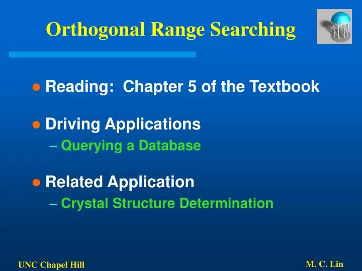
Orthogonal Range Searching. Reading: Chapter 5 of the Textbook Driving Applications Querying a Database Related Application Crystal Structure Determination. Interprete DB Queries Geometrically. Transform records in database into points in multi-dimensional space.

E N D
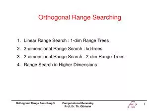
Orthogonal Range Searching • Reading: Chapter 5 of the Textbook • Driving Applications • Querying a Database • Related Application • Crystal Structure Determination M. C. Lin
Interprete DB Queries Geometrically • Transform records in database into points in multi-dimensional space. • Transform queries on d-fields of records in the database into queries on this set of points in d-dimensional space. • A query asking to report all records whose fields lie between specific values trans-forms to a query asking for all points inside a d-dimensional axis-parallel box. M. C. Lin
1-D Range Searching • Let P := {p1, p2, …, pn} be a given set of points on the real line. A query asks for the points inside a 1-D query rectangle -- i.e. an interval [x:x’] • Use a balanced binary search tree T. The leaves of T store the points of P and the internal nodes of T store splitting values to guide the search. Let the splitting value at a node v be xv. The left subtree of v contains all points xv and the right subtree of v contains all points > xv. • To report points in [x:x’], we search with x and x’ in T. Let u and u’ be the two leaves where the search ends resp. Then the points in [x:x’] are the ones stored in leaves between u and u’, plus possibly points stored at u & u’. M. C. Lin
FindSplitNode(T, x, x’) Input: A tree T and two values x and x’ with x x’ Output: The node v where the paths tox and x’ splits, or the leaf where both paths end. 1. v root (T) 2. while v is not a leaf and (x’ xv or x > xv) 3. do if x’ xv 4. then v lc(v) (* left child of the node v *) 5. else v rc(v) (* right child of the node v *) 6. return v M. C. Lin
1DRangeQuery(T, [x:x’]) Input: A range tree T and a range [x:x’] Output: All points that lie in the range. 1. vsplit FindSplitNode(T, x, x’) 2. ifvsplitis a leaf 3. then Check if the point stored at vsplit must be reported 4. else (* Follow the path to x and report the points in subtrees right of the path *) 5. v lc(vsplit) M. C. Lin
1DRangeQuery(T, [x:x’]) 6. while v is not a leaf 7. do if x xv 8. then ReportSubTree(rc(v)) 9. v lc(v) 10. else v rc(v) 11. Check if the point stored at leaf v must be reported 12. Similarly, follow the path to x’, report the points in subtrees left of the path, and check if point stored at the leaf where the path ends must be reported. M. C. Lin
1D-Range Search Algorithm Analysis • Let P be a set of n points in one-dimensional space. The set P can be stored in a balanced binary search tree, which uses O(n) storage and has O(n log n) construction time, s.t. the points in a query range can be reported in time O(k + log n), where k is the number of reported points. • The time spent in ReportSubtree is linear in the number of reported points, i.e. O(k). • The remaining nodes that are visited on the search path of x or x’. The length is O(log n) and time spent at each node is O(1), so the total time spent at these nodes is O(log n). M. C. Lin
Kd-Trees • A 2d rectangular query on P asks for points from P lying inside a query rectangle [x:x’] x [y:y’]. A point p:= (px, py) lies inside this rectangle iff px [x:x’] and py [y:y’]. • In 2D case, there are two important values: its x- and y- coordinates. Thus, we first split on x-coordinate, next on y-coordinate, then again on x-coordinate, and so on. • At the root, we split P with l into 2 sets and store l. Each set is then split into 2 subsets and stores its splitting line. We proceed recursively as such. • In general, we split with vertical lines at nodes whose depth is even, and split with horizontal lines at nodes whose depth is odd. M. C. Lin
BuildKDTree(P, depth) Input: A set P of points and the current depth, depth. Output: The root of kd-tree storing P. 1. ifPcontains only 1 point 2. then return a leaf storing at this point 3. else if depth is even 4. then Split P into 2 subsets with a vertical line l thrumedian x-coordinate of points in P. Let P1 and P2 be the sets of points to the left or on and to the right of l respectively. 5. else Split P into 2 subsets with a horizontal line l thrumedian y-coordinate of points in P. Let P1 and P2 be the sets of points below or on l and above l respectively. 5. vleft BuildKDTree(P1, depth + 1) 6.vright BuildKDTree(P2, depth + 1) 7. Create a node vstoring l, make vleft & vright lef/right children of v 8. return v M. C. Lin
Construction Time Analysis • The most expensive step is median finding, which can be done in linear time. • T(n) = O(1), if n = 1 • T(n) = O(n) + 2 T(n/2), if n > 1 T(n) = O(n logn) • A kd-tree for a set of n points uses O(n) storage and can be constructed in O(nlogn) time. M. C. Lin
Querying on a kd-Tree • In general, region corresponding to a node v is a rectangle, or region(v), which can be unbounded on 1 sides. It’s bounded by splitting lines stored at ancestors of v. A point is stored in the sub-tree rooted at v if and only if it lies in region(v). • We traverse the kd-tree, but visit only nodes whose region is intersected by the query rectangle. When a region is fully contained in the query rectangle, we report all points stored in its sub-trees. When the traversal reaches a leaf, we have to check whether the point stored at the leaf is contained in the query region. M. C. Lin
SearchKDTree(v, R) Input: The root of a (subtree of a) kd-tree and a range R. Output: All points at leaves below v that lie in the range. 1. ifvis a leaf 2. then Report the point stored at v if it lies in R. 3. else if region(lc(v)) is fully contained in R 4. then ReportSubtree(lc(v)) 5. else if region(lc(v)) intersects R 6. then SearchKDTree(lc(v), R) 7. If region(rc(v)) is fully contained in R 8. then ReportSubtree(rc(v)) 9. else if region(rc(v)) intersects R 10. then SearchKDTree(rc(v), R) M. C. Lin
2D KD-Tree Query Time Analysis • The time to traverse a subtree and report points in its leaves is linear in the number of reported points. • To bound the number of other nodes visited, we bound the number of regions intersected by edges of the query rectangle. • Q(n) = O(1), if n = 1 • Q(n) = 2 + 2 Q(n/4), if n > 1 Q(n) = O(n1/2) M. C. Lin
KD-Tree Query Time Analysis • A rectangle range query on the kd-tree for a setof n points in the plane takes O(n1/2+k) time, where k is number of reported points. • A d-dimensional kd-tree for a set of n points takes O(d·n) storage and O(d ·nlogn) time to construct. The query time is bounded by O(n1-1/d + k). M. C. Lin
Basics of Range Trees • Similar to 1D, to report points in [x:x’] x [y:y’], we search with x and x’ in T. Let u and u’ be the two leaves where the search ends resp. Then the points in [x:x’] are the ones stored in leaves between u and u’, plus possibly points stored at u & u’. • Call the subset of points stored in the leaves of the subtree rooted at v, the canonical subset of v. For the root, it’s whole set P; for a leave, it’s the point stored there. • We can perform the 2D range query similarly by only visiting the associated binary search tree on y-coordinate of the canonical subset of v, whose x-coordinate lies in the x-interval of the query rectangle. M. C. Lin
Range Trees • The main tree is a balanced binary search tree T built on the x-coordinate of the points in P. • For any internal or leaf node v in T, the canonical subset of P(v) is stored in a balanced binary search tree Tassoc(v) on the y-coordinate of the points. The node v stores a pointer to the root of Tassoc(v), which is called the “associated structure” of v. This is called a “Range Tree”. The DS where nodes have pointers to associated structures are often called multi-level data structures. The main tree T is then called the first-level tree and the associated structures are second-level trees. M. C. Lin
Build2DRangeTree(P) Input: A set P of points in the plane. Output: The root of 2-dimensional tree. 1. Build a binary search tree Tassoc on the set Py of y-coordinates of the points in P. Store at leaves of Tassoc the points themselves. 2. ifPcontains only 1 point 3. then Create a leaf v storing this point and make Tassoc the associated structure of v. 4. else Split P into 2 subsets: Pleft containing points with x-coordinatexmid, the median x-coordinate, and Pright containing points with x-coordinatexmid 5. vleft Build2DRangeTree(Pleft) 6.vright Build2DRangeTree(Pright) 7. Create a node vstoring xmid, make vleft left child of v & vright right child of v, and makeTassoc the associated structure of v 8. return v M. C. Lin
2DRangeQuery(T, [x:x’] x [y:y’]) Input: A 2D range tree T and a range [x:x’] x [y:y’] Output: All points in T that lie in the range. 1. vsplit FindSplitNode(T, x, x’) 2. ifvsplitis a leaf 3. then Check if the point stored at vsplit must be reported 4. else (* Follow the path to x and call 1DRangeQuery on the subtrees right of the path *) 5. v lc(vsplit) M. C. Lin
2DRangeQuery(T, [x:x’] x [y:y’]) 6. while v is not a leaf 7. do if x xv 8. then 1DRangeQuery(Tassoc(rc(v)), [y:y’]) 9. v lc(v) 10. else v rc(v) 11. Check if the point stored at leaf v must be reported 12. Similarly, follow the path from rc(vsplit) to x’, call 1DRangeQuery with the range [y:y’] on the associated structures of subtrees left of the path, and check if point stored at the leaf where the path ends must be reported. M. C. Lin
Range Tree Algorithm Analysis • Let P be a set of n points in the plane. A range tree for P uses O(n log n) storage and can be constructed in O(n log n) time. By querying this range tree, one can report the points in P that lie in a rectangular query range in O(log2n + k) time, where k is the number of reported points. M. C. Lin
Higher-D Range Trees • Let P be a set of n points in d-dimensional space, where d 2. A range tree for P uses O(nlogd-1n) storage and it can be constructed in O(nlogd-1n) time. One can report the points in P that lies in a rectangular query range in O(logdn + k) time, where k is the number of reported points. M. C. Lin
General Sets of Points • Replace the coordinates, which are real numbers, by elements of the so-called composite-number space. The elements of this space are pair of reals, denoted by (a|b). We denote the order by: (a|b) < (a’|b’) a < a’ or (a=a’ and b<b’) • Many points are distince. But for the ones with same x- or y-coordinate, replace each point p :=(px, py) by p’ :=((px| py), (py| px)) • Replace R:=[x:x’] x [y:y’] by R’ := [(x| -) : (x’| + )] x [(y| -) : (y’| + )] M. C. Lin
Basics of Fractional Cascading • Both P(lc(v)) and P(rc(v)) are canonical subsets of P(v). Each canonical subset P(v) is stored in an associated structure. Instead of using a binary search tree, we now store it in an array A(v). The array is sorted on the y-coordinate of the points. Each entry in A(v) stores 2 pointers: a pointer into A(lc(v)) & a pointer into A(rc(v)). • A(v)[i] stores a point p :=(px ,py ). We store a pointer from A(v)[i] to the entry of A(lc(v)) s.t. the y-coordinate of p’ stored there is the smallest one py. The pointer to A(rc(v)) is defined the same way: it points to the entry s.t. the y-coordinate of the point stored there is the smallest one that is py. This modified version is called “layered range tree”. M. C. Lin
Fractional Cascading Algorithm Analysis • Let P be a set of n points in d-dimensional space, with d 2. A layered range tree for P uses O(nlogd-1n) storage and it can be constructed in O(nlogd-1n) time. With this range tree, one can report the points in P that lies in a rectangular query range in O(logd-1n + k) time, where k is the number of reported points. M. C. Lin