Download
1 / 48
490 likes | 599 Views
Variational and Geometric Aspects of Compatible Discretizations . May 12, 2004 Pavel Bochev Computational Mathematics and Algorithms Sandia National Laboratories. Supported in part by.

E N D
Variational and Geometric Aspectsof Compatible Discretizations May 12, 2004 Pavel Bochev Computational Mathematics and Algorithms Sandia National Laboratories Supported in part by Sandia is a multiprogram laboratory operated by Sandia Corporation, a Lockheed Martin Company,for the United States Department of Energy’s National Nuclear Security Administration under contract DE-AC04-94AL85000.
1950 + 50 = 2000 It’s about time ! Why are we here? We conclude…that exterior calculus is here to stay, that it will gradually replace tensor methods in numerous situations where it is the more natural tool, that it will find more and more applications because of its inner simplicity. Physicists are beginning to realize its usefulness; perhaps it will soon make its way into engineering. H. Flanders, 1963 There’s generally a time lag of some fifty years between mathematical theories and their applications…
Acknowledgments and Sources • Thanks to • D. Arnold (IMA) • M. Gunzburger (FSU) • R. Lehoucq (SNL) • R. Nicolaides (CMU) • A. Robinson (SNL) • M. Shashkov (LANL) • C. Scovel (LANL) • K. Trapp (CMU) • Variational methods • A. Aziz, et al. (1972) • G. Strang and G. Fix, (1973) • F. Brezzi, RAIRO B-R2 (1974) • G. Fix, M. Gunzburger, R. Nicolaides, CMA 5, (1979) • F. Brezzi, C. Bathe, CMAME 82, (1990) • F. Brezzi, M. Fortin, Mixed FEM, Springer (1991) • Direct/geometric methods • J. Dodzuik, (1976) • M. Hyman, J. Scovel, LAUR (1988-92) • M. Hyman, M. Shashkov, S. Stenberg (1995-98) • R. Nicolaides, SINUM 29 (1992) • K. Trapp Ph.D Thesis (2004) • Connections • R. Kotiuga, PhD Thesis, (1984), PIERS32 (2001) • A. Bossavit, IEEE Trans Mag.18 (1988) • C. Mattiussi, JCP (1997) • L. Demkowicz, TICAM99-06, (1999) • R. Hiptmair, Numer. Math., 90 (2001), PIERS32 • D. Arnold, ICM, Beijing, (2002)
Variational Energy principle Direct System equilibrium Differential Model - reduce the admissible states - apply the same principle - find the reduced state that fits best the exact system - reduce the system - apply the same physics - find the exactstate of the reduced system How different people discretize Physics Discretization is a model reduction that replaces a physical process by a parametrized family of algebraic equations.
What do we want to know? 1. Is the sequence of algebraic equations well-behaved? - are all problems uniquely and stably (in h) solvable? - do solutions converge to the exact solutions as h0? 2. Are physical and discrete models compatible? - are solutions physically meaningful - do they mimic, e.g., invariants, symmetries of actual states 3. How to make a compatible & accurate discretization? - how to choose the variables and where to place them; - how to avoid spurious solutions. We revisit earlier discussion with a particular focus on how - variational compatibility (Arnold) - geometric compatibility (Nicolaides, Shashkov) can be used to answer these questions.
Solvability Stability Stability of linear systems arising from PDEs cannot be assessed by standard condition number: A sequence of linear systems vs. a single linear system
The smallest generalized singular value of Kh must bebounded away from zero, independent of h. Stability of a sequence glb suggested by G. Golub stability = and are independent of h
Galerkin theorem solvability stability approximation + Variational compatibility Unique solvability and quasi-optimal convergence Variational Methods Galerkin approximation of operator equations
FEM = variational principle + piecewise polynomial subspaces Projection Quasi-projection Variational settings for FEM Optimization No optimization
Examples No Optimization - Advection-Diffusion-Reaction models - Navier-Stokes equations Constrained Optimization Kelvin principle: - the solenoidal velocity field that minimizes kinetic energy is irrotational Dirichlet principle: - the irrotational velocity field that minimizes kinetic energy is solenoidal Unconstrained Optimization - Poisson equation
No Optimization Variational problem Unique solvability & stability X continuity Inf-sup (I) Y Inf-sup (II)
Xh continuity conformity: Yh Inf-sup (I) Inf-sup (II) Compatibility Discrete problem Variational compatibility Necessary but insufficient!
Constrained Optimization Variational problem Z V Unique solvability & stability continuity of a and b coercivity on Z S inf-sup for B
Zh Compatibility Discrete Problem V Vh Z Variational compatibility continuity conformity Necessary but insufficient: Sh S
coercivity on Zh inf-sup for Bh Variational compatibility V Vh conformity Z Zh Sh S
Vh conformity: continuity & coercivity! Unconstrained Optimization Variational problem Unique solvability & stability continuity V coercivity Discrete problem Variational compatibility
Allows to assert powerful results about the asymptotic behavior • quasi-optimal error estimates • unique solvability for any h • stability of discrete solutions (uniform invertibility ) This answers the 1st question: 1. Is the family of algebraic equations well-behaved? - are all problems uniquely and stably (in h) solvable? - do solutions converge to the exact solutions as h 0? What does variational compatibility buy you Sequence stability is equivalent to variational compatibility
What does variational compatibility say about the other issues? Not much Variational compatibility conditions are not constructive! • These conditions are not very helpful in finding the stable spaces and may be difficult to verify. Creative application of non-trivial tricks required, e.g., • Fortin’s operator • Verfurth’s method • Boland & Nicolaides’s method • Inf-sup fear and loathing still common!
Kinematic relation Continuity relation Constitutive equation “Pure” Direct Discretizations Algebraic model Reduced system u12 u11 p9 p7 p8 u9 u10 u8 u7 u6 p6 p4 p5 u3 u4 u5 u2 u1 p3 p1 p2
The Hodge A possible “physical” interpretation of Hodge: (Franco’s question) Conversion of velocity (measured along a line) into a flow (measured across a surface)
Note that if we were to build the reduced system, its behavior will be described exactly by this algebraic equation! Matrix Form Kinematic Constitutive Continuity
Differential forms provide the tools to encode such relationships • Integration: an abstraction of the measurement process • Differentiation: gives rise to local invariants • Poincare Lemma: expresses local geometric relations • Stokes Theorem: expresses global relations (differentiation + integration) Geometric compatibility Geometrically compatible discretization: algebraic equations that describe “actual” physical systems. Requires to discover structure and invariants of physical systems and then copy them to a discrete system • Fields are observed indirectly by measuring global quantities (flux, circulation, etc) • Physical laws are relationships between global quantities (conservation, equilibrium)
System states are differential forms reduced to co-chains Exterior differentiation approximated by the co-boundary operator Dual operators defined using Hodge * operator Branin (1966), Dodzuik (1976), Hyman & Scovel (1988-92), Mattiussi (1997), Teixeira (2001) Mimetic and co-volume methods fit this reduction model • Vector fields represented by their integrals (fluxes or circulations) • Differential operators defined via Stokes Theorem (coordinate-invariant) • Primal and dual equations/operators (B and BT) and an inner product (A) How to achieve geometric compatibility? Algebraic topology provides the tools to copy the structure
Commuting Diagram I Fundamental property: Algebraic Topology Approach 1. System reduction 3 exact sequences:(W0, W1, W2, W3), (C0, C1, C2, C3), (C0, C1, C2, C3) forms co-chains DeRham map chains {G,D,C} approximates d {grad,curl,div}
Example chains = 0 co-chains = 0
Commuting Diagram II Algebraic Topology Approach 2. Inner products and dual operators Inner product Inner product Dual operators G*, C*, D* C*G*=D*C*=0requires
Examples Co-volume Mimetic Whitney Nicolaides, Trapp (1992-04) Hyman, Shashkov, Steinberg (1985-04) Dodzuik (1976) Hyman, Scovel (1988)
Approximation (Shashkov, Wheeler, Yotov 2004/ Trapp, 2004) (Dodzuik, 1976) Properties • Co-volume inner product is the unique inner product that is • diagonal • exact for constant vector fields Important computational property: • dual co-volume operators have localstencils Action of co-volume and mimetic products coincides if Stencil of D* (Trapp, 2004)
Geometric compatibility CDP 1 CDP 2 Algebraic Topology Framework: Summary • Structures: (W0, W1, W2, W3) Forms (C0, C1, C2, C3) Chains (C0, C1, C2, C3) Co-chains • De Rham map • Interpolation operator • Inner product • Primal and dual operators {G,C,D} & {G*,C*,D*}
Examples: Co-volume:Nicolaides et. al. 1992-2004 Finite difference:Yee, 1966 Finite volume:Weiland, 1977 Direct discretization of a div-curl system
Eliminations Examples Mimetic:Shashkov et. al. 1995-2004 Finite volume: The box integration method: Mock, 1983 Direct discretization of a div-grad system
What does geometric compatibility buy you? Co-cycles of (W0, W1, W2, W3) co-cycles of (C0, C1, C2, C3) Discrete Poincare lemma (existence of potentials in contractible domains) Discrete Stokes Theorem Discrete “Vector Calculus” CG = DC = 0; C*G* = D*C* = 0 Any feature of the continuum system that is implied by differential forms calculus is inherited by the discrete model Called mimeticproperty by Hyman and Scovel (1988)
Unique solvability: Assume: surjection CDP I surjection , a contradiction! Solvability: free of charge Div-curl system: Discrete Helmholtz orthogonality Div-grad system: Commuting diagram property
Variational • Operator-centric point of view • Problem = operator equation on function spaces • Discretization = operator equation + functional approximation • Stability conditions • Error estimates Geometric • Topology-centric point of view • Problem = equilibrium relation on manifolds • Discretization = equilibrium relation + manifold approximation • Forces physically compatible discretization patterns • Preserves problem structure Variational vs. geometric stability conditions not constructive - do not reveal structure of stable discretizations
I will now examine connections between geometrical and variational compatibility that validate such collaborations using Kelvin’s principle as a prototype problem Variational and geometric We can benefit from combining both approaches D. Arnold stable mixed spaces designed by association of the problem with a differential complex M. Shashkov error analysis of mimetic schemes enabled by identification with a mixed Galerkin method and a proper quadrature selection.
geometry GDP metric Theorem GDP is necessary and sufficient for stable, optimally accurate mixed discretization of the Kelvin principle. Fix, Gunzburger, Nicolaides, ICASE Report 78-7, 1977, Num. Math, 1981 Early examples Grid Decomposition Property Helmholtz Similar GDP exists for the Dirichlet principle but is trivial to satisfy!
(Vh,Sh) verify inf-sup condition for the Kelvin principle iff: geometry metric equivalent to a commuting diagram! Early examples Fortin Lemma Geometric assumption: Douglas and Roberts, Math. Appl. Comp. 1982
Can this be an accident? • We see : • conditions that combine geometric and metric properties • the ubiquitous commuting diagram… TheFrench Connection Bossavit, Nedelec, Verite, 1982-88 and Kotiuga, 1984, were first from the finite element community to notice and document an uncanny connection between unusual, i.e., not nodal, finite element spaces and Whitney forms.
Variational compatibility Forms DOFs FEMs CDP CDP 1 + CDP 2 = VC Geometric compatibility CDP 1 CDP 2 CDP is equivalent to stability of mixed FEM CDP and GDP are also equivalent!
Co-volume Mimetic Whitney, 1957 simplex Nedelec, 1980-85 cube, prism Van Welij, 1985 hexahedron BD(F)M, 80s -90s many shapes FEM There’s only one low-order compatible method Well, up to a choice of an inner product… And a quadrature rule… And a cell shape… FEM shapes restricted to those that have a “reference element”!
Allows to automate formulation of high-order spaces: • Define reference space containing desired polynomials • Glue together into piecewise polynomial space • Coordinate interpolation and DOFs to provide CDP There are more high-order methods But they are mostly FEM….Why? • Direct methods: • reliance on the De Rham map limits DOFs to co-chains: stencils expand! • Variational methods: • order = degree of complete polynomials contained in the space (Bramble-Hilbert) Demkowicz et. al. TICAM Report (1999), Hiptmair’s talk, PIERS 32 (2001), Arnold & Winther Numer. Math. (2002), Winther’s talk
Conclusions • Stronger in metric-dependent aspects : • assessment of the asymptotic behavior (error, stability) • formulation of higher-order methods • Weaker in structure-dependent aspects: • compatibility conditions not constructive, difficult to verify • FEM restricted to special cell shapes Variational: • Weaker in metric-dependent aspects : • uniform stability of systems, errors, harder to prove • higher-order methods not easy to define directly • Stronger in structure-dependent aspects: • structure of the problem copied automatically • local/global relationships and invariants preserved • admit a wider set of cell shapes Geometric:
Conclusions Variational +Geometric is better Enjoy the workshop!
Another viewpoint Recall the discrete network of pipes… Constitutive • Kinematic and continuity relations • depend only on “network topology” • (incidence matrices!) • Metric is introduced by • the constitutive equation. Kinematic Continuity This distinct pattern appears over and over in physical models (Tonti, 1974). It can be used to provide an additional insight into compatible discretizations
“All” 2nd order PDE’s K=1 • One DDF set used • One set eliminated • One d is exact • One d is weak • One grid only • Typical: • Mixed FEM • Mimetic FD • Two DDF sets used • Two d’s are exact • Two grids (P&D) • Typical: • Co-Volume • Staggered grid De Rham complex Discrete De Rham complex Discrete factorization diagram Primal Hodge topology topology Dual Elimination “All”MethodsPrimal-dual Factorization diagram Primal metric Hodge h topology topology Dual Factorization (Tonti) diagrams metric Tonti (1974), PIERS 32 (2001), Bossavit IEEE Mag. (1988), Hiptmair Num. Math. (2001)