Transaction Processing

1. Transaction Processing Chapter 16

2. Transaction Concept • A transactionis a unit of program execution that accesses and possibly updates various data items. • A transaction must see a consistent database. • During transaction execution the database may be inconsistent. • When the transaction is committed, the database must be consistent. • Two main issues to deal with: • Failures of various kinds, such as hardware failures and system crashes • Concurrent execution of multiple transactions

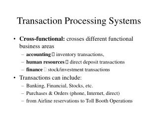
3. Transactions • Concurrent execution of user programs is essential for good DBMS performance. • Because disk accesses are frequent, and relatively slow, it is important to keep the cpu humming by working on several user programs concurrently. • A user’s program may carry out many operations on the data retrieved from the database, but the DBMS is only concerned about what data is read/written from/to the database. • A transactionis the DBMS’s abstract view of a user program: a sequence of reads and writes.

4. Example of Fund Transfer • Transaction to transfer $50 from account A to account B: read(A) A := A – 50 write(A) read(B) B := B + 50 write(B) • Transaction to increase the amount in account A by $100. read(A) A := A + 100 write(A)

5. Concurrency in a DBMS • Users submit transactions, and can think of each transaction as executing by itself. • Concurrency is achieved by the DBMS, which interleaves actions (reads/writes of DB objects) of various transactions. • Each transaction must leave the database in a consistent state if the DB is consistent when the transaction begins. • DBMS will enforce some ICs, depending on the ICs declared in CREATE TABLE statements. • Beyond this, the DBMS does not really understand the semantics of the data. (e.g., it does not understand how the interest on a bank account is computed). • Issues:Effect of interleaving transactions, and crashes.

6. Example • Consider two transactions (Xacts): T1: BEGIN A=A+100, B=B-100 END T2: BEGIN A=1.06*A, B=1.06*B END • Intuitively, the first transaction is transferring $100 from B’s account to A’s account. The second is crediting both accounts with a 6% interest payment. • There is no guarantee that T1 will execute before T2 or vice-versa, if both are submitted together. However, the net effect must be equivalent to these two transactions running serially in some order.

7. Example (Contd.) • Consider a possible interleaving (schedule): T1: A=A+100, B=B-100 T2: A=1.06*A, B=1.06*B • This is OK. But what about: T1: A=A+100, B=B-100 T2: A=1.06*A, B=1.06*B • The DBMS’s view of the second schedule: T1: R(A), W(A), R(B), W(B) T2: R(A), W(A), R(B), W(B)

8. Anomalies with Interleaved Execution • Reading Uncommitted Data (WR Conflicts, “dirty reads”): • Unrepeatable Reads (RW Conflicts): T1: R(A), W(A), R(B), W(B), Abort T2: R(A), W(A), C T1: R(A), R(A), W(A), C T2: R(A), W(A), C

9. Anomalies (Continued) • Overwriting Uncommitted Data (WW Conflicts, “lost update problem” ): • Incorrect summary problem: T1: W(A), W(B), C T2: W(A), W(B), C T1: R(A), R(B), R(X), R(Y), ..., T2: R(X), W(X), R(Y), W(Y), C

10. Transaction State • Active, the initial state; the transaction stays in this state while it is executing • Partially committed, after the final statement has been executed. • Failed, after the discovery that normal execution can no longer proceed. • Aborted, after the transaction has been rolled back and the database restored to its state prior to the start of the transaction. Two options after it has been aborted: • restart the transaction – only if no internal logical error • kill the transaction • Committed, after successful completion.

11. Transaction State (Cont.)

12. The Log • The following actions are recorded in the log: • Ti writes an object: the old value and the new value. • Log record must go to diskbeforethe changed page! • Ti commits/aborts: a log record indicating this action. • Log records are chained together by Xact id, so it’s easy to undo a specific Xact. • Log is often duplexed and archived on stable storage. • All log related activities (and in fact, all CC related activities such as lock/unlock, dealing with deadlocks etc.) are handled transparently by the DBMS.

13. The ACID Properties • Atomicity: All actions in the Xact happen, or none happen. • Consistency: If each Xact is consistent, and the DB starts consistent, it ends up consistent. • Isolation: Execution of one Xact is isolated from that of other Xacts. • Durability: If a Xact commits, its effects persist.

14. Passing the ACID Test • Logging and Recovery • Guarantees Atomicity and Durability. • Concurrency Control • Guarantees Consistency and Isolation, given Atomicity.

15. Schedules • Schedule: An interleaving of actions from a set of Xacts, where the actions of any one xact are in the original order. • Represents some actual sequence of database actions. • Example: R1(A), W1(A), R2(B), W2(B), R1(C), W1(C) • In a complete schedule, each Xact ends in commit or abort.

16. Acceptable Schedules • One sensible “isolated, consistent” schedule: • Run Xacts one at a time, in a series. • This is called a serial schedule. • NOTE: Different serial schedules can have different final states; all are “OK” -- DBMS makes no guarantees about the order in which concurrently submitted Xacts are executed. • Serializable schedules: • Final state is what some serial schedule would have produced. • Aborted Xacts are not part of schedule; ignore them for now (they are made to `disappear’ by using logging).

17. Example Schedules • Let T1 transfer $50 from A to B, and T2 transfer 10% of the balance from A to B. The following is a serial schedule, in which T1 is followed by T2. Schedule 1

18. Example Schedule (Cont.) • Let T1 and T2 be the transactions defined previously. The following schedule is not a serial schedule, but it is equivalent to the previous Schedule. Schedule 2 In both Schedule 1 and 2, the sum A + B is preserved.

19. Example Schedules (Cont.) • The following concurrent schedule does not preserve the value of the sum A + B. Schedule 3

20. Serializability • Basic Assumption – Each transaction preserves database consistency. • Thus serial execution of a set of transactions preserves database consistency. • A (possibly concurrent) schedule is serializable if it is equivalent to a serial schedule. • Different forms of schedule equivalence give rise to the notions of: 1. conflict serializability 2. view serializability • We ignore operations other than read and write instructions, and we assume that transactions may perform arbitrary computations on data in local buffers in between reads and writes. Our simplified schedules consist of only read and write instructions.

21. Conflict Serializability • Instructions li and lj of transactions Ti and Tj respectively, conflict if and only if there exists some item Q accessed by both li and lj, and at least one of these instructions wrote Q. 1. li = read(Q), lj = read(Q). li and ljdon’t conflict.2. li = read(Q), lj = write(Q). They conflict.3. li = write(Q), lj = read(Q). They conflict4. li = write(Q), lj = write(Q). They conflict • Intuitively, a conflict between liand lj forces a (logical) temporal order between them. If li and lj are consecutive in a schedule and they do not conflict, their results would remain the same even if they had been interchanged in the schedule.

22. Conflict Serializability (Cont.) • If a schedule S can be transformed into a schedule S´ by a series of swaps of non-conflicting instructions, we say that S and S´ are conflict equivalent. • We say that a schedule S is conflict serializable if it is conflict equivalent to a serial schedule • Example of a schedule that is not conflict serializable: T3T4read(Q)write(Q)write(Q)We are unable to swap instructions in the above schedule to obtain either the serial schedule < T3, T4 >, or the serial schedule < T4, T3 >.

23. Conflict Serializability (Cont.) • Schedule 2 below can be transformed into Schedule 1, a serial schedule where T2 follows T1, by series of swaps of non-conflicting instructions. Therefore Schedule 2 is conflict serializable.

24. Example Schedule (Schedule A) T1 T2 T3 T4 T5 read(X)read(Y)read(Z) read(V) read(W) read(W) read(Y) write(Y) write(Z)read(U) read(Y) write(Y) read(Z) write(Z) read(U)write(U)

25. T1 T2 Precedence Graph • A Precedence (or Serializability) graph: • Node for each commited Xact. • Arc from Ti to Tj if an action of Ti precedes and conflicts with an action of Tj. • T1 transfers $100 from A to B, T2 adds 6% • R1(A), W1(A), R2(A), W2(A), R2(B), W2(B), R1(B), W1(B)

26. Test for Conflict Serializability • A schedule is conflict serializable if and only if its precedence graph is acyclic. • Cycle-detection algorithms exist which take order n2 time, where n is the number of vertices in the graph. (Better algorithms take order n + e where e is the number of edges.) • If precedence graph is acyclic, the serializability order can be obtained by a topological sorting of the graph. This is a linear order consistent with the partial order of the graph.

27. Precedence Graph for Schedule A T1 T2 T4 T3 A serializability order for Schedule A would beT5 T1 T3 T2 T4 .

28. View Serializability • Let S and S´ be two schedules with the same set of transactions. S and S´ are view equivalentif the following three conditions are met: 1. For each data item Q, if transaction Tireads the initial value of Q in schedule S, then transaction Ti must, in schedule S´, also read the initial value of Q. 2. For each data item Q if transaction Tiexecutes read(Q) in schedule S, and that value was produced by transaction Tj(if any), then transaction Ti must in schedule S´ also read the value of Q that was produced by transaction Tj . 3. For each data item Q, the transaction (if any) that performs the final write(Q) operation in schedule S must perform the finalwrite(Q) operation in schedule S´. • As can be seen, view equivalence is also based purely on reads and writes alone.

29. View Serializability (Cont.) • A schedule S is view serializable if it is view equivalent to a serial schedule. • Every conflict serializable schedule is also view serializable. • A schedule which is view-serializable but not conflict serializable. • Every view serializable schedule that is not conflict serializable has blind writes.

30. Test for View Serializability • The precedence graph test for conflict serializability must be modified to apply to a test for view serializability. • The problem of checking if a schedule is view serializable falls in the class of NP-complete problems. Thus existence of an efficient algorithm is unlikely. • However practical algorithms that just check some sufficient conditions for view serializability can still be used.

31. Other Notions of Serializability • Schedule given below produces same outcome as the serial schedule <T1,T5 >, yet is not conflict equivalent or view equivalent to it. • Determining such equivalence requires analysis of operations other than read and write.

32. Concurrency Control vs. Serializability Tests • Testing a schedule for serializability after it has executed is a little too late! • Goal – to develop concurrency control protocols that will assure serializability. They will generally not examine the precedence graph as it is being created; instead a protocol will impose a discipline that avoids nonseralizable schedules. • Tests for serializability help understand why a concurrency control protocol is correct.

33. Now, Aborted Transactions • Serializable schedule: Equivalent to a serial schedule of committed Xacts. • as if aborted Xacts never happened. • Two Issues: • How does one undo the effects of a xact? • We’ll cover this in logging/recovery • What if another Xact sees these effects?? • Must undo that Xact as well!

34. Recoverable Schedules • Abort of T1 requires abort of T2! • But T2 has already committed! • A recoverable schedule is one in which this cannot happen. • i.e. a Xact commits only after all the Xacts it “depends on” (i.e. it reads from or overwrites) commit. • Real systems typically ensure that only recoverable schedules arise (through locking).

35. Cascading Aborts • Abort of T1 requires abort of T2! • Cascading Abort • What about WW conflicts & aborts? • T2 overwrites a value that T1 writes. • T1 aborts: its “remembered” values are restored. • Lose T2’s write! • An ACA (avoids cascading abort) schedule is one in which cascading abort cannot arise. • A Xact only reads/writes data from committed Xacts. • Every cascadeless schedule is also recoverable. • Strict Schedule: Xacts only read/write changes of committed Xacts.