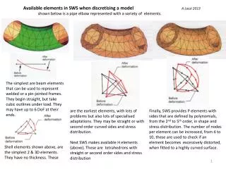
Available elements in SWS when discretising a model A Lozzi 2013

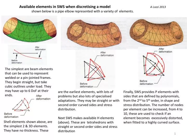
1. Available elements in SWS when discretising a model A Lozzi 2013 shown below is a pipe elbow represented with a variety of elements. The simplest are beam elements that can be used to represent welded or a pin-jointed frames. They begin straight, but take cubic outlines under load. They may have up to 6 DoF at their ends. are the earliest elements, with lots of problems but also lots of specialised adaptations. They may be straight or with second order curved sides and stress distribution. Next SWS makes available H elements (above). These are tetrahedrons with straight or second order sides and stress distribution Finally, SWS provides P elements with sides that are defined by polynomials, from the 2nd to 5thorder, in shape and stress distribution. The number of nodes per element can be increased, from 4 to 10, these are used to check if an element becomes excessively distorted, when fitted to a highly curved surface. Shell elements shown above, are the simplest 2 & 3D elements. They have no thickness. These

4. Defaults element size, usually very effective H elements. P elements with curved edges Allowed variation in element size. Number of element around a circle. Variation in size of adjacent elements. Allows the mesher to search for largest element size that will mesh fully

5. H elements vary in size, P elements can vary in size and polynomial order

6. Note that the deformation plot, at left, show changes in all edge shapes, except for the restrained left face. This produces errors at that end of the plate. We could have defined equal and opposite forces on left and right faces, then using ‘soft springs’ to balance the numerical errors in the final calculations.

7. It is possible to sections through the Stress plot. Von Mises and principal stresses are available, showing pure tension at the surface at right, compression pressure between surfaces in contact.

8. Default mesh shown above. Note there is 2 elements through the thickness of the plate Top left shows an example of probing, Large element size limit the ability to pick the highest stress location. But, the table shows that 7 fold increase in number of elements does not have a huge effect in this case on the calculated highest stress. For most components the default mesh size is very effective and you do not have to grow old waiting for an answer.

9. The available options on colour range and numerical precision are shown. Note that from the previous example , it is obvious that to quote stress to more than 2 significant figures is just misleading.

10. A model with a perfectly sharp corner, in principle produces infinitely high stress at that corner. Hence higher and higher mesh density results in higher and higher maximum stress, as is shown on table below. If a malleable material like low carbon steels were used, then yielding at the corner would result in formation of a fillet. A brittle material would develop a crack from the corner. SW advises that uncertainty of the ‘true’ stresses are caused least by modelling, most by unrealistic fixtures. Uncertainty (errors) in material properties is at least in the order of 5% from reputable suppliers, which is further degraded by surface and internal defects, during manufacture. Consider then the total uncertainty in the actual stresses in a particular component.

13. All contacts between parts in an assembly (ie top level) are by default presumed to be bonded. Each pair of contacting surfaces may be changed to ‘no penetration’ or other, by progressively selecting and redefining them. Contacting faces may be automatically detected by using: Tools/Interference detection/Options - select treat coincidence as interference – calculate.

14. Selection of solver methods Direct Sparse arrives at exact solutions . Good for models of 100,000 DoF or less. FFFPlus is an iterative method, better for larger models and multiple contacts. Automatic, allows the system to chose the solver. Adaptive methods allows the system to iterate to reach acceptable errors. Very slow and requires experience to apply reasonably Soft Spring - surrounds the model with relatively very soft restraints. Inertial Relief – adds equal and opposite forces to any small unbalanced resultant.

15. SW in one of their training courses, uses the bracket shown at left as an example of their Adaptive mesh capability. Presumably they put this forward as an exemplary application of the use of Adaptive mesh generation, but I think it could be improved upon. At top is the model of finished part. Below it is the simplified model which is meshed. Note – the chamfers on all outer edges are removed because convex corners do not increase stress. Their removal will make the model simpler and quicker. The fillet at the T junction must be kept because this will generate stress concentration. The back surface has been reshaped by flattening it. The fillets on the rear face would caused higher than average stresses, but they are now removed. Also the stress at the front fillets will now be enhanced because they now are closer to a fixed face, than they had originally been.

16. The P adaptive mesh generation, left the mesh size and distribution as originally developed. This method increased the variation of edge and stress distribution within the elements to the maximum 5th order polynomial. The H method refined the mesh in areas of high stress, to about 1/10th their original size.

17. What are the true stresses ? Possibly the most accurate estimation was obtained by photo elastic studies using near clear plastics and polarised light. Many of these studies support the stress concentration factors seen at the back of many references. Typically today’s FEA do not produce the resolution comparable with those of past polarised light studies.