Download
1 / 71
730 likes | 999 Views
The AS-AD model. From the short run to the medium run. In the short run prices are either sticky (non moving) or adjusting very slowly. We can say that their adjustment is sluggish. Output can be above or below its natural level.

E N D
From the short run to the medium run • In the short run prices are either sticky (non moving) or adjusting very slowly. We can say that their adjustment is sluggish. Output can be above or below its natural level. • In the medium run prices are flexible. They adjust over time. Output returns to its natural level, the level determined by an economy’s productive capacity, i.e. the amount of its factors of production (capital and labor).
From the short run to the medium run • So far, by using the IS-LM model, we have a picture of the demand side of the economy. • To get to the medium run we also need to get a picture of the supply side of the economy.
The Labor market • To get to the supply side, we need to take into account the labor market. • In the labor market, we will identify two forces that determine the equilibrium level of the real wage and the equilibrium level of unemployment. • We will call these forces: the wage setting relation and the price setting relation.
The Labor market (Wage setting) • Who sets the wages in the labor market? • Who else, the interested parties: employers and employees. • How do they set the prices? • They bargain, either individually or collectively through unions. • Why do they do it like that? • Well, there is no other way in a decentralized economy.
The Labor market (Wage setting) • So, as employees, how would decide what nominal wage offer to float on the negotiations table? • Wouldn’t we take into account the price level that we would expect to face in the future? Yes, we would. We would like to be insured against changes in the price level for the time that the wage contract would bind us. So our offer would depend on the expected price level (Pe).
The Labor market (Wage setting) • Our offer would also depend on the conditions of the labor market. If there is high unemployment, we would be willing to settle for a lower wage because the chances of finding another job are slim. However, if there is low unemployment, then we can take our chances and ask for a high wage since we can find another job easily. • So our wage offer depends negatively on the rate of unemployment (u).
The Labor market (Wage setting) • Finally, our offer depends on other factors that affect the labor market, like e.g. unemployment benefits. The higher they are, the higher wage we will ask. Or another factor could be the power of the union we belong in and the solidarity of its members. • We will call these other factors z and we will assume that our wage offer depends positively on them. The higher they are, the more money we ask.
The Labor market (Wage setting) • Of course, our employers think in the same way. The higher they expect the price level to be, the higher nominal wage they would be willing to give. The higher they observe the unemployment rate to be, the lower wage they are going to offer. The higher the unemployment benefits and the other factors are, the higher their offer is going to be.
The Labor market (Wage setting) • Since both parties, employees and employers base their decisions on the same factors, the wage setting decision they are going to reach will depend on these factors as well. • The nominal wage will depend one to one on the expected price level Pe. It will also depend on the unemployment rate u and the other factors z. Since we don’t know how exactly it depends on u and z, we will include those in a function that will call F(u,z). • Therefore, mathematically we write: W = PeF(u, z) • This is the wage setting relation.
The Labor market (Price setting) • Now, how do the firms determine the price they are going to sell their goods at? • Well, for starters there is a simple rule: they wouldn’t want to sell at a price that is less than their cost. • But what is their cost? • By assumption, firms only use labor. So, they produce according to a production function that looks like that: Y = F(N) • Output is a function of the labor N employed. • What if we make a further assumption: every worker that firms employ produces only one good. In that case, the production function becomes even simpler: Y = N
The Labor market (Price setting) • Next step: how much do firms pay their workers? • The answer is easy: they pay them the nominal wage W. • Now, if we assume that we are in a perfect competition environment, where firms make zero profits, then it must be that firms sell each good for a price P that is equal to the nominal wage W. • Remember each worker produces one good and firms pay this worker W. Then firms break even if they sell each good for P = W.
The Labor market (Price setting) • Now, if we assume away perfect competition and allow firms to make some profits, then the firms may charge a price that is above the nominal wage that they pay to the workers. • We call the amount that the price exceeds the nominal wage, markup and we denote it by μ. • Mathematically we write: P = (1 + μ)W • This is the price setting relation and it tells us that P is greater than W by a factor μW. The firms now make profits and our scenario is more realistic.
The Labor market (Wage and Price setting combined) • We can make an assumption that will simplify things bit, namely that in the wage setting relation, the nominal wage depends not on the expected price level but on the actual price level. • This could be because e.g. workers negotiate wages very often (say every month). In that case, they wouldn’t need to form expectations about the price level because since they would renegotiate their wage very soon.
The Labor market (Wage and Price setting combined) • So, if Pe = P, the wage setting relation becomes: W = PF(u, z) • Solving for the real wage W/P, we obtain: W/P = F(u, z) • This expression tells us that the real wage W/P is negatively related to unemployment u and positively related to the other factors z.
The Labor market (Wage and Price setting combined) • Also solving the price setting relation for the real wage we obtain: P = (1 + μ)W => P/W = (1 + μ) => W/P = 1/(1 + μ) • This expression tells us that the real wage W/P does not depend on unemployment but only on the markup μ.
The Labor market (Wage and Price setting combined) • If we equate the two expressions for the real wage that we obtained from the wage and the price setting relations we obtain: F(un, z) = 1/(1 + μ) • When the real wage is in equilibrium, we say that unemployment is at its natural rate, which we denote by un.
The Labor market in equilibrium Here we combine the wage setting relation, which tells us that the real wage is a negative function of the unemployment rate, and the price setting relation, which tells us that the real wage does not depend on unemployment. When the labor market clears we obtain the equilibrium level of real wage and the equilibrium rate of unemployment, which we call the natural rate of unemployment. W/P 1/(1 +μ) PS WS un u
Deriving the AS curve • Now that we have described the labor market, we can combine the wage setting and the price setting relation to get an expression between prices and output. • Let’s start from the price setting equation P = (1 + μ)W and let’s substitute the wage with its equal from the wage setting equation W = PeF(u,z) • We obtain P = Pe(1 + μ)F(u, z).
Deriving the AS curve • Furthermore: u = U/L => u = (L – N)/L => u = L/L – N/L => u = 1 – N/L But according to our production function Y=N. Therefore: u = 1 – Y/L
Deriving the AS curve • Substituting this expression for u into the expression that we obtained before, we get: P = Pe(1 + μ)F(1 – Y/L, z), which is the AS relation. • This expression shows a positive relationship between output and prices. • We will now explain why.
Deriving the AS curve • If output goes up then unemployment goes down. • If unemployment goes down, workers are in a better bargaining position and can ask for higher nominal wages (remember the wage setting equation). • If nominal wages go up, this means that the firms have to charge higher prices to cover their increased costs (remember the price setting equation). • Therefore higher output leads to higher prices and we have established the positive relationship between the two variables.
Deriving the AS curve P Starting from the labor market we have managed to establish a positive relationship between output and prices. The AS curve depicts this relationship. AS Y
Deriving the AD curve • Let’s return to the IS-LM model and let’s see what happens if we assume an increase in prices. • The increase in prices means that the supply of real money balances decreases shifting the LM curve to the left (up). This results in a lower level of output.
Deriving the AD curve • Therefore a higher level of prices, through the IS-LM model, leads to a lower level of output. • We call this negative relationship between prices and output AD relation and mathematically we express it as: Y = Y(G, T, M/P) • This means that output depends on G, T and M/P. • In particular any change of these factors that shifts the IS or the LM to the right (or to the left), also shifts the AD curve to the right (or to the left).
Deriving the AD curve P Starting from an increase in prices in Panel A, the supply of real money balances M/P goes down. This shifts the LM curve to the left (up) leading to a lower level of output. Therefore, we have established that a higher level of output, through the IS-LM model translates to a lower level of output. The AD curve in Panel B sums up this negative relationship between prices and output. P2 Panel B P1 AD Y2 Y1 Y i LM2 Panel A LM1 i2 B i1 A IS Y2 Y1 Y
Combining the AS and AD curves P Combining the AS and AD curves we may find the equilibrium level of prices and output in an economy. AS P* AD Y* Y
Fiscal expansion • As we already know, a fiscal expansion is a situation where the government increases government expenditures (G). This is synonymous to an increase in the government deficit (G - T). • As we have mentioned, this corresponds to a shift of the IS curve to the right. • If we assume that we start at the natural level of output (Yn), the result of the shift is a level of output higher than the natural level and a higher level of interest rate.
Fiscal expansion • Turning to the AS-AD model, the shift of the IS curve to the right means that the AD curve also shifts to the right. This leads to a higher level of prices. Prices now exceed the expected level of prices. Remember that by definition, when output is at the natural level, actual prices are equal to expected prices. Now, we are at our new short run equilibrium (point B). Output and prices are higher compared to the initial level.
Fiscal expansion • Moving from the short to the medium run, since prices rose, wage setters, who are not idiotic, will increase their price expectations. In turn, this increase in expected prices will shift the AS curve upward, so actual prices will rise again. • The process starts again: wages setters adjust their price expectations shifting the AS curve up and increasing actual prices. • The process comes to an end, when output, moving along the new AD curve returns to its natural level. When output reaches again its natural level, wage setters have no reason to adjust their expectations and the spiral price increase ends. Now, we are at our new medium run equilibrium (point C). Output is the same compared to the initial level but prices are higher.
Fiscal expansion • We have to take one final step to complete our experiment: turn back to the IS-LM model. • The rise in prices that occurred from the short run to the medium run means that the supply of real money balances (M/P) decreased. This means that the LM curve will shift to the left (up). It will keep shifting left (up) until output reaches its previous natural level (point C). The interest rate now is even higher.
Fiscal expansion Starting at the natural level of output, an initial increase in G shifts the IS to the right in Panel A. This results in a level of output higher than the natural level and a higher interest rate. In Panel B the AD curve shifts to the right leading to higher output and actual prices higher than the expected level. The short run equilibrium is at point B in both panels. Over time, the higher prices induce wage setters to increase their price expectations shifting up the AS curve in Panel B. Shifting stops at the new medium run equilibrium at point C along the new AD curve, where output is back to its initial natural level and prices are higher. Back to Panel A, the increase in prices reduces the supply of real money balances shifting the LM curve to the left (up). In the medium run we end up at point C, back to the natural level of output but with a higher interest rate. P AS2 Panel B P’e =P3 C AS1 P2 B Pe =P1 A AD2 AD1 Yn Y1 Y i LM2 Panel A i3 C LM1 i2 B i1 A IS2 IS1 Yn Y1 Y
Fiscal expansion in the short run • So now, we have a clear picture of how all our variables moved in the short run compared to their initial level: • Y: output is positively affected. It rises above its natural level. • C: consumption is positively affected since our disposable income increases. • i: the interest rate increases. • I: the movement of investment is ambiguous because on the one hand output went up and we know that this boosts I, but on the other hand the interest rate increased and we also know that this shrinks investment. So the net effect is ambiguous. • P: prices increase. • u: unemployment rate goes down, below its natural level, since output goes up and we need more people employed to produce that. • G: government expenditures go up by assumption.
Fiscal expansion in the medium run • We also have a clear picture of how all our variables moved in the medium run compared to their initial level: • Y: output goes back to its natural level. It is unchanged compared to the initial level. • C: consumption is also unchanged since output is unchanged. • i: the interest rate increases. • I: investment unambiguously decreases because the interest rate increased, while output is unchanged. So only the negative effect of the interest rate increase is at work. • P: prices increase. • u: unemployment rate is unchanged since we are back to the previous level of output. • G: government expenditures go up by assumption. Notice that investment goes down by as much as G goes up in order for output to be unchanged. This is the well known crowding out effect.
Fiscal contraction • A fiscal contraction is a situation where the government decreases government expenditures (G). This is synonymous to a decrease in the government deficit (G - T). • As we have mentioned, this corresponds to a shift of the IS curve to the left. • If we assume that we start at the natural level of output (Yn), the result of the shift is a level of output lower than the natural level and a lower level of interest rate.
Fiscal contraction • Turning to the AS-AD model, the shift of the IS curve to the left means that the AD curve also shifts to the left. This leads to a lower level of prices. Prices now are below the expected level of prices. Now, we are at our new short run equilibrium (point B). Output and prices are lower compared to the initial level.
Fiscal contraction • Moving from the short to the medium run, since prices fell, wage setters will decrease their price expectations. In turn, this decrease in expected prices will shift the AS curve downward, so actual prices will fall again. • The process starts again: wages setters adjust their price expectations shifting the AS curve down and decreasing actual prices. • The process comes to an end, when output, moving along the new AD curve returns to its natural level. When output reaches again its natural level, wage setters have no reason to adjust their expectations and the spiral price decrease ends. Now, we are at our new medium run equilibrium (point C). Output is the same compared to the initial level but prices are lower.
Fiscal contraction • Going back to the IS-LM model, the fall in prices that occurred from the short run to the medium run means that the supply of real money balances (M/P) increased. This means that the LM curve will shift to the right (down). It will keep shifting right (down) until output reaches its previous natural level (point C). The interest rate now is even lower.
Fiscal contraction Starting at the natural level of output, an initial decrease in G shifts the IS to the left in Panel A. This results in a level of output lower than the natural level and a lower interest rate. In Panel B the AD curve shifts to the left leading to lower output and actual prices lower than the expected level. The short run equilibrium is at point B in both panels. Over time, the lower prices induce wage setters to decrease their price expectations shifting down the AS curve in Panel B. Shifting stops at the new medium run equilibrium at point C along the new AD curve, where output is back to its initial natural level and prices are lower. Back to Panel A, the decrease in prices increases the supply of real money balances shifting the LM curve to the right (down). In the medium run we end up at point C, back to the natural level of output but with a lower interest rate. P Panel B AS1 Pe =P1 A AS2 P2 B P’e =P3 C AD1 AD2 Y1 Yn Y i LM1 Panel A i1 A LM2 i2 B i3 C IS1 IS2 Y1 Yn Y
Fiscal contraction in the short run • So now, we have a clear picture of how all our variables moved in the short run compared to their initial level: • Y: output is negatively affected. It falls below its natural level. • C: consumption is negatively affected since our disposable income decreases. • i: the interest rate decreases. • I: the movement of investment is ambiguous because on the one hand output went down and we know that this lowers I, but on the other hand the interest rate decreased and we also know that this boosts investment. So the net effect is ambiguous. • P: prices decrease. • u: unemployment rate goes up, above its natural level, since output goes down and we need less people employed to produce that. • G: government expenditures go down by assumption.
Fiscal contraction in the medium run • We also have a clear picture of how all our variables moved in the medium run compared to their initial level: • Y: output goes back to its natural level. It is unchanged compared to the initial level. • C: consumption is also unchanged since output is unchanged. • i: the interest rate decreases. • I: investment unambiguously increases because the interest rate decreased, while output is unchanged. So only the positive effect of the interest rate decrease is at work. • P: prices decrease. • u: unemployment rate is unchanged since we are back to the previous level of output. • G: government expenditures go down by assumption. Notice that investment goes up by as much as G goes down in order for output to be unchanged.
Monetary expansion • We already know that a monetary expansion is a situation where the central bank increases the money supply. • We also know that this shifts the LM curve to the right (down). • The result is a higher a level of output and a lower level of interest rate.
Monetary expansion • Turning to the AS-AD model, the shift of the LM curve to the right means that the AD curve also shifts to the right. This leads to a higher level of prices. Prices now exceed the expected level of prices. Now, we are at our new short run equilibrium (point B). Output and prices are higher compared to the initial level.
Monetary expansion • Moving from the short to the medium run, since prices rose, wage setters will increase their price expectations. In turn, this increase in expected prices will shift the AS curve upward, so actual prices will rise again. • The process starts again: wages setters adjust their price expectations shifting the AS curve up and increasing actual prices. • The process comes to an end, when output, moving along the new AD curve returns to its natural level. When output reaches again its natural level, wage setters have no reason to adjust their expectations and the spiral price increase ends. Now, we are at our new medium run equilibrium (point C). Output is the same compared to the initial level but prices are higher.
Monetary expansion • Going back to the IS-LM model, the rise in prices that occurred from the short run to the medium run means that the supply of real money balances (M/P) decreased. This means that the LM curve will shift to the left (up). It will keep shifting left (up) until output reaches its previous natural level, back to point A. The interest rate returns to its previous level.
Monetary expansion Starting at the natural level of output, an initial increase in money supply shifts the LM to the right (down) in Panel A. This results in a level of output higher than the natural level and a lower interest rate. In Panel B the AD curve shifts to the right leading to higher output and actual prices higher than the expected level. The short run equilibrium is at point B in both panels. Over time, the higher prices induce wage setters to increase their price expectations shifting up the AS curve in Panel B. Shifting stops at the new medium run equilibrium at point C in Panel B along the new AD curve, where output is back to its initial natural level and prices are higher. Back to Panel A, the increase in prices reduces the supply of real money balances shifting the LM curve back to the left (up). In the medium run in Panel A, we end up back at point A, back to the natural level of output but with the same interest rate compared to the initial level. P AS2 Panel B P’e =P3 C AS1 P2 B Pe =P1 A AD2 AD1 Yn Y1 Y i Panel A LM1 i1 A LM2 i2 B IS Yn Y1 Y