Download
1 / 29
300 likes | 320 Views
Dynamic Optimization and Automatic Differentiation. Yi Cao School of Engineering Cranfield University. Outline. Dynamic optimization problems Parameterization Recursive high-order Taylor series ODE and sensitivity solver Dynamic optimization solver Differential recurrent neural network

E N D
Dynamic Optimization and Automatic Differentiation Yi Cao School of Engineering Cranfield University Colloquium on Optimization for Control
Outline • Dynamic optimization problems • Parameterization • Recursive high-order Taylor series • ODE and sensitivity solver • Dynamic optimization solver • Differential recurrent neural network • Continuous-time NMPC • Conclusions Colloquium on Optimization for Control
Dynamic optimization problem • Controller design, =const controller parameter • Adaptive control, =variable controller parameter • System identification, =model parameter • Predictive control, =control action, variable • State estimation, =initial state • …… Colloquium on Optimization for Control
Solving dynamic optimization • Optimal control theory well established in 1960s. • Challenge for numerical solutions: • Complex / large scale problems • Efficiency for realtime optimization • Global optimization • Stability • Robustness Colloquium on Optimization for Control
Differentiation and dynamic optimization • H=Φ(t,x,)+λ’f(t,x,) • Optimal conditions: dx/dt= Hλ=f(t,x,), dλ/dt=–Hx=–Φx(t,x,)–fx(t,x,)λ H=Φ(t,x,)+f(t,x,)λ=0 • Efficient solution requires efficient differentiation Colloquium on Optimization for Control
Differentiation approaches • Analytic differentiation manually Not a trivial task for large scale problem • Analytic differentiation using symbolic computing software Very complicated results even for a small problem • Numerical finite difference Inefficient and inaccurate Colloquium on Optimization for Control
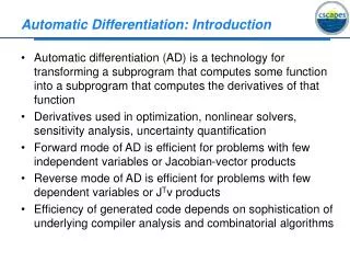
Automatic Differentiation (1) • Techniques use computer programs to get derivatives of any functions represented in other computer programs with the same accuracy and efficiency as the function. • Synonym: Algorithmic Differentiation • First proposed by Johnannes Joos, 1976 in his PhD Thesis, ETH, Zurich Colloquium on Optimization for Control
Automatic Differentiation (2) • Factor: every computer program, no matter how complicated, executes a sequence of elementary arithmetic operations such as additions or elementary functions such as exp(). • By applying the chain rule of derivative calculus repeatedly to these operations, derivatives of arbitrary order can be computed automatically, and accurate to working precision. Colloquium on Optimization for Control
Automatic Differentiation (3) Two modes to calculate derivatives: • Forward mode: y=f(x(t)) • Reverse mode (adjoint): y=f(x(t)) Colloquium on Optimization for Control
Automatic Differentiation (4) Two ways to implement AD • Operator overloading Each elementary operation is replaced by a new one, working on pairs of value and its derivative (doublet). • Source transformation Produce new code to calculate derivative based on original code of a function Colloquium on Optimization for Control
AD Example: Forward Mode y=sin(x1/x2)+x1/x2–exp(x2) x1’=1, x2’=0 v1’=(x1’x2-x1x2’)/x2/x2=2 v2’=cos(v1)*v1’= –1.98 v3’=exp(x2)*x2’=0 v4’=v1’-v3’=2 y’=v2’+v4’=0.02 x1=1.5, x2=0.5 v1=x1/x2=3 v2=sin(v1)=0.1411 v3=exp(x2)=1.649 v4=v1–v3=1.3513 y=v2+v4=1.4924 Colloquium on Optimization for Control
AD Example: Reverse Mode y=sin(x1/x2)+x1/x2–exp(x2) x2=x2+v1*x1/x2/x2=-1.589 x1=v1/x2=0.02 v1=v2*cos(v1)+v1=0.01 x2=v3*exp(x2)=-1.649 v1=v4=1, v3=–v4=–1 y=1, v2=y=1, v4=y=1 x1=1.5, x2=0.5 v1=x1/x2=3 v2=sin(v1)=0.1411 v3=exp(x2)=1.649 v4=v1–v3=1.3513 y=v2+v4=1.4924 Colloquium on Optimization for Control
Automatic Taylor expansion • z(t)=f(x(t)), t scalar, x and z vectors • TS: x(t)=x0+x1t+x2t2+…+xdtd • TS: z(t)=z0+z1t+z2t2+…+zdtd • AD forward (TS of z): zk = zk(x0,x1,…,xk) • AD reverse (TS of sensitivity): zk /xj = zk-j / x0 := Ak-j • f’x=A0+A1t+A2t2+…+Adtd Colloquium on Optimization for Control
Recursively solving ODE using TS • dx/dt=f(x) • dx/dt=z(t) • Recursive relation: xk+1=zk/(k+1). • x0=x(t0), • x1=z0(x0), • x2=z1(x0,x1), … • x(t0+h)=di=0 xihi • Next step: t1=t0+ht0 Colloquium on Optimization for Control
Solving ODE with sensitivity equation • Sensitivity equation: dx/dt=fx(t,x,)x+f(t,x,) • v={x0,} • Avk:=zk/v • Bvk:=dxk/dv • Bvk+1= (Avk+kj=0Axk-jBvj)/(k+1) • Bv:=dx(t0+h)/dv =Bv0+Bv1h+Bv2h2+…+Bvdhd Colloquium on Optimization for Control
Solving dynamic optimization using TS • Convert cost to terminal cost: min F(tf,x(tf),(tf)) • Initial guass: 0={0(t0),…, 0(tf)} • Step: hi=ti+1-ti>0, i=0,1,…,n-1, tn=tf • Integrate ODE & sensitivity from t0 to tf • x(t0), x(t1), …, x(tf) and F(tf,x(tf),0(tf)) • Bx(t1),…,Bx(tf), B(t1),…,B(tf) and Fx, F • dF/d0(ti)=FxBx(tf)…Bx(ti+2)B(ti+1) • For constant , dF/d0= dF/d0(ti) • Update i+1=i- dF/di Colloquium on Optimization for Control
Error Control • h=step, d=order of TS • (h,d)=C(h/r)d+1 • r ≈ rd=||xd-1||/||xd|| for large d • (h,d-1) ≈(h,d)(rd/h)≤(h,d)+||xd|| • (h,d)≤h||xd||2/(||xd-1||-h||xd||) • Given tolerance and d, determine h • Given tolerance, determine optimal d, h to minimize computation. • Global error: ≥||Bx||i and g global tolerance • local tolerance: =g(-1)/(n-1) Colloquium on Optimization for Control
NMPC using differential recurrent NN • Continuous-time nonlinear identification • Efficient algorithm to train DRNN • Training performance and efficiency • DRNN as internal model for NMPC • Efficient algorithm for NMPC • NMPC performance and efficiency Colloquium on Optimization for Control
Differential recurrent neural networks Colloquium on Optimization for Control
DRNN Training • ={b1,b2,vec(W2),vec(W1x),vec(W1u)} • N=Nh+Nx+Nh×Nu+2Nh×Nx • Training data: u(t), y(t) at t=0,h,…,Nh • Solving DRNN + sensitivity using TS • Assume t=0 is steady-state, apply u(t) • y(t) at t=h,…,Nh and ek=y(kh)-y(kh) • minkeTkek/2=ETE/2, E=vec(e1,…,eN) • Nonlinear least square (NLSQ) optimization Colloquium on Optimization for Control
Continuous time NMPC • minu φ=∫0T(y-yr)TQ(y-yr)+(u-ur)TR(u-ur)dt/2 • s.t. dx/dt=f(x,u), y=g(x) • umin≤ u ≤ umax, 0=t0 ≤ … ≤ tP=T • Parameterize u: piecewise polynomial • u(t)=qi=0uki(t-tk)i tk ≤ t ≤ tk+1, k=0,…,P-1 • U=[uT00,…,uT0q,…,uTP-10,…,uTP-1q]T • Y=[yT00,…,yT0d,…,yTP-10,…,yTP-1d]T • φ=T(YeTHQYe+UeTHRUe)/2 • φ=ETE/2 NLSQ Colloquium on Optimization for Control
NMPC algorithm (with DRNN) • x0 (steady-state or estimated), ym • d=ym-Cx0 (constant for 0 ≤ t ≤ T) • U0 Ue=U0-Ur X Y Ye=Y-Yr+d • Jacobian, J=E/U • Unconstrained: Uk+1=Uk-(JTJ)-1JTE • Input constrained: lsqnonlin • Other constraints: fmincon/SQP • Apply [uT00,…,uT0q]T • repeat Colloquium on Optimization for Control
Tank Reactor Example • 2-CSTR in series, reaction A+B C • 2-output: T1 and T2 ,2-input: Qcw1 and Qcw2 • Distuabnce: Tcw • 6 states Colloquium on Optimization for Control
DRNN identification • Nh=6, Nx=6, Nu=2, N=96 • 600-s data with h=0.1 s, N=6000 • Total sensitivity 3456000 • Validation set sampled at 0.02 s • Advantage: change sampling rate does not need re-training Colloquium on Optimization for Control
Training and Validating Colloquium on Optimization for Control
Training efficiency (one epoch) Colloquium on Optimization for Control
NMPC performance, setpoint change Colloquium on Optimization for Control
NMPC performance, disturbance rejection Colloquium on Optimization for Control
Conclusions • High-order TS using AD • Efficiently solving ODE + sensitivity • Efficient algorithm for general dynamic optimization • Efficient algorithm for RDNN training • Efficient algorithm for continuous-time NMPC • Demonstrated with 2-CSTR example. Colloquium on Optimization for Control