Download
1 / 46
470 likes | 479 Views
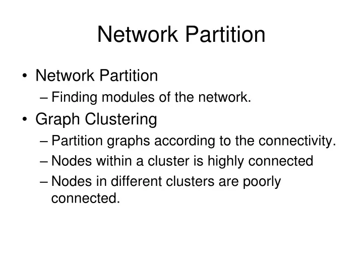
Network Partition. Network Partition Finding modules of the network. Graph Clustering Partition graphs according to the connectivity. Nodes within a cluster is highly connected Nodes in different clusters are poorly connected. Applications. It can be applied to regular clustering

E N D
Network Partition • Network Partition • Finding modules of the network. • Graph Clustering • Partition graphs according to the connectivity. • Nodes within a cluster is highly connected • Nodes in different clusters are poorly connected.
Applications • It can be applied to regular clustering • Each object is represented as a node • Edges represent the similarity between objects • Chameleon uses graph clustering. • Bioinformatics • Partition genes, proteins • Web pages • Communities discoveries
Challenges • Graph may be large • Large number of nodes • Large number of edges • Unknown number of clusters • Unknown cut-off threshold
Graph Partition • Intuition: • High connected nodes could be in one cluster • Low connected nodes could be in different clusters.
A Partition Method based on Connectivities • Cluster analysis seeks grouping of elements into subsets based on similarity between pairs of elements. • The goal is to find disjoint subsets, called clusters. • Clusters should satisfy two criteria: • Homogeneity • Separation
Introduction • In similarity graph data vertices correspond to elements and edges connect elements with similarity values above some threshold. • Clusters in a graph are highly connected subgraphs. • Main challenges in finding the clusters are: • Large sets of data • Inaccurate and noisy measurements
Important Definitions in Graphs Edge Connectivity: • It is the minimum number of edges whose removal results in a disconnected graph. It is denoted by k(G). • For a graph G, if k(G) = l then G is called an l-connected graph.
Important Definitions in Graphs A B A B D C D C Example: GRAPH 1 GRAPH 2 The edge connectivity for the GRAPH 1 is 2. The edge connectivity for the GRAPH 2 is 3.
Important Definitions in Graphs Cut: • A cut in a graph is a set of edges whose removal disconnects the graph. • A minimum cut is a cut with a minimum number of edges. It is denoted by S. • For a non-trivial graph G iff |S| = k(G).
Important Definitions in Graphs A B A B D C D C Example: GRAPH 1 GRAPH 2 The min-cut for GRAPH 1 is across the vertex B or D. The min-cut for GRAPH 2 is across the vertex A,B,C or D.
Important Definitions in Graphs Distance d(u,v): • The distance d(u,v) between vertices u and v in G is the minimum length of a path joining u and v. • The length of a path is the number of edges in it.
Important Definitions in Graphs Diameter of a connected graph: • It is the longest distance between any two vertices in G. It is denoted by diam(G). Degree of vertex: • Its is the number of edges incident with the vertex v. It is denoted by deg(v). • The minimum degree of a vertex in G is denoted by delta(G).
Important Definitions in Graphs A B D C E Example: d(A,D) = 1 d(B,D) = 2 d(A,E) = 2 Diameter of the above graph = 2 deg(A) = 3 deg(B) = 2 deg(E) = 1 Minimum degree of a vertex in G = 1
Important Definitions in Graphs Highly connected graph: • For a graph with vertices n > 1 to be highly connected if its edge-connectivity k(G) > n/2. • A highly connected subgraph (HCS) is an induced subgraph H in G such that H is highly connected. • HCS algorithm identifies highly connected subgraphs as clusters.
Important Definitions in Graphs A B Not HCS! D C E Example: No. of nodes = 5 Edge Connectivity = 1
Important Definitions in Graphs A B HCS! D C Example continued: No. of nodes = 4 Edge Connectivity = 3
HCS Algorithm HCS(G(V,E)) begin (H, H’,C) MINCUT(G) if G is highly connected then return (G) else HCS(H) HCS(H’) end if end
HCS Algorithm • The procedure MINCUT(G) returns H, H’ and C where C is the minimum cut which separates G into the subgraphs H and H’. • Procedure HCS returns a graph in case it identifies it as a cluster. • Single vertices are not considered clusters and are grouped into singletons set S.
HCS Algorithm Example
HCS Algorithm Example Continued
HCS Algorithm Example Continued Cluster 2 Cluster 1 Cluster 3
HCS Algorithm • The running time of the algorithm is bounded by 2N*f(n,m). N - number of clusters found f(n,m) – time complexity of computing a minimum cut in a graph with n vertices and m edges • Current fastest deterministic algorithms for finding a minimum cut in an unweighted graph require O(nm) steps.
Properties of HCS Clustering Diameter of every highly connected graph is at most two. That is any two vertices are either adjacent or share one or more common neighbors. This is a strong indication of homogeneity.
Properties of HCS Clustering Each cluster is at least half as dense as a clique which is another strong indication of homogeneity. Any non-trivial set split by the algorithm has diameter at least three. This is a strong indication of the separation property of the solution provided by the HCS algorithm.
Modified HCS Algorithm Example
Modified HCS Algorithm Example – Another possible cut
Modified HCS Algorithm Example – Another possible cut
Modified HCS Algorithm Example – Another possible cut
Modified HCS Algorithm Example – Another possible cut Cluster 1 Cluster 2
Modified HCS Algorithm Iterated HCS: • Choosing different minimum cuts in a graph may result in different number of clusters. • A possible solution is to perform several iterations of the HCS algorithm until no new cluster is found. • The iterated HCS adds another O(n) factor to running time.
Modified HCS Algorithm Singletons adoption: • Elements left as singletons can be adopted by clusters based on similarity to the cluster. • For each singleton element, we compute the number of neighbors it has in each cluster and in the singletons set S. • If the maximum number of neighbors is sufficiently large than by the singletons set S, then the element is adopted by one of the clusters.
Modified HCS Algorithm Removing Low Degree Vertices: • Some iterations of the min-cut algorithm may simply separate a low degree vertex from the rest of the graph. • This is computationally very expensive. • Removing low degree vertices from graph G eliminates such iteration and significantly reduces the running time.
Modified HCS Algorithm HCS_LOOP(G(V,E)) begin for (i = 1 to p) do remove clustered vertices from G H G repeatedly remove all vertices of degree < d(i) from H
Modified HCS Algorithm until(no new cluster is found by the HCS call) do HCS(H) perform singletons adoption remove clustered vertices from H end until end for end
Key features of HCS Algorithm • HCS algorithm was implemented and tested on both simulated and real data and it has given good results. • The algorithm was applied to gene expression data. • On ten different datasets, varying in sizes from 60 to 980 elements with 3-13 clusters and high noise rate, HCS achieved average Minkowski score below 0.2.
Key features of HCS Algorithm • In comparison greedy algorithm had an average Minkowski score of 0.4. Minkowski score: • A clustering solution for a set of n elements can be represented by n x n matrix M. • M(i,j) = 1 if i and j are in the same cluster according to the solution and M(i,j) = 0 otherwise. • If T denotes the matrix of true solution, then Minkowski score of M = ||T-M|| / ||T||
Key features of HCS Algorithm • HCS manifested robustness with respect to higher noise levels. • Next, the algorithm were applied in a blind test to real gene expression data. • It consisted of 2329 elements partitioned into 18 clusters. HCS identified 16 clusters with a score of 0.71 whereas Greedy got a score of 0.77.
Key features of HCS Algorithm • Comparison of HCS algorithm with Optimal • Graph theoretic approach to data clustering
Summary Clusters are defined as subgraphs with connectivity above half the number of vertices Elements in the clusters generated by HCS algorithm are homogeneous and elements in different clusters have low similarity values Possible future improvement includes finding maximal highly connected subgraphs and finding a weighted minimum cut in an edge-weighted graph.
Graph Clustering Intuition: High connected nodes could be in one cluster Low connected nodes could be in different clusters. Model: A random walk may start at any node Starting at node r, if a random walk will reach node t with high probability, then r and t should be clustered together.
Markov Clustering (MCL) • Markov process • The probability that a random will take an edge at node u only depends on u and the given edge. • It does not depend on its previous route. • This assumption simplifies the computation.
MCL • Flow network is used to approximate the partition • There is an initial amount of flow injected into each node. • At each step, a percentage of flow will goes from a node to its neighbors via the outgoing edges.
MCL • Edge Weight • Similarity between two nodes • Considered as the bandwidth or connectivity. • If an edge has higher weight than the other, then more flow will be flown over the edge. • The amount of flow is proportional to the edge weight. • If there is no edge weight, then we can assign the same weight to all edges.
Intuition of MCL • Two natural clusters • When the flow reaches the border points, it is likely to return back, then cross the border. A B
MCL • When the flow reaches A, it has four possible outcomes. • Three back into the cluster, one leak out. • ¾ of flow will return, only ¼ leaks. • Flow will accumulate in the center of a cluster (island). • The border nodes will starve.