Download
1 / 36
360 likes | 444 Views
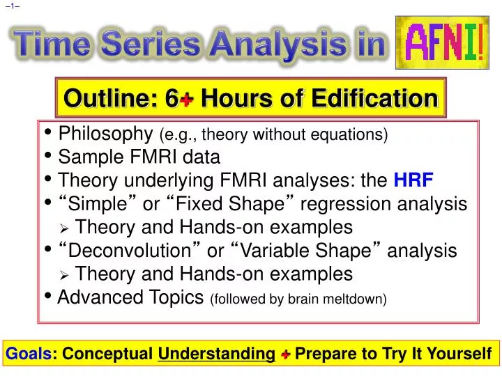
Time Series Analysis in. Outline: 6 + Hours of Edification. Philosophy (e.g., theory without equations) Sample FMRI data Theory underlying FMRI analyses: the HRF “ Simple ” or “ Fixed Shape ” regression analysis Theory and Hands-on examples

E N D
Time Series Analysis in Outline: 6+ Hours of Edification • Philosophy (e.g., theory without equations) • Sample FMRI data • Theory underlying FMRI analyses: the HRF • “Simple” or “Fixed Shape” regression analysis • Theory and Hands-on examples • “Deconvolution” or “Variable Shape” analysis • Theory and Hands-on examples • Advanced Topics (followed by brain meltdown) Goals: Conceptual Understanding+ Prepare to Try It Yourself
Data Analysis Philosophy • Signal = Measurable response to stimulus • Noise = Components of measurement that interfere with detection of signal • Statistical detection theory: • Understand relationship between stimulus & signal • Characterize noise statistically • Can then devise methods to distinguish noise-only measurements from signal+noise measurements, and assess the methods’ reliability • Methods and usefulness depend strongly on the assumptions • Some methods are more “robust” against erroneous assumptions than others, but may be less sensitive
FMRI Philosopy: Signals and Noise • FMRI StimulusSignalconnection and noise statistics are both complex and poorly characterized • Result: there is no “best” way to analyze FMRI time series data: there are only “reasonable” analysis methods • To deal with data, must make some assumptions about the signal and noise • Assumptions will be wrong, but must do something • Different kinds of experiments require different kinds of analyses • Since signal models and questions you ask about the signal will vary • It is important to understand what is going on, so you can select and evaluate “reasonable” analyses
Meta-method for creating analysis methods • Write down a mathematical model connecting stimulus (or “activation”) to signal • Write down a statistical model for the noise • Combine them to produce an equation for measurements given signal+noise • Equation will have unknown parameters, which are to be estimated from the data • N.B.: signal may have zero strength (no “activation”) • Use statistical detection theory to produce an algorithm for processing the measurements to assess signal presence and characteristics • e.g., least squares fit of model parameters to data
Time Series Analysis on Voxel Data • Most common forms of FMRI analysis involve fitting an activation+BOLD model to each voxel’s time series separately(“massively univariate” analysis) • Some pre-processing steps do include inter-voxel computations; e.g., • spatial smoothing to reduce noise • spatial registration to correct for subject motion • Result of model fits is a set of parameters at each voxel, estimated from that voxel’s data • e.g., activation amplitude (β), delay, shape • “SPM”=statistical parametric map; e.g., β or t or F • Further analysis steps operate on individual SPMs • e.g., combining/contrasting data among subjects • sometimes called “second level” or “meta” analysis
Some Features of FMRI Voxel Time Series • FMRI only measures changes due to neural “activity” • Baseline level of signal in a voxel means little or nothing about neural activity • Also, baseline level tends to drift around slowly (100 s time scale or so; mostly from small subject motions) • Therefore, an FMRI experiment must have at least 2 different neural conditions (“tasks” and/or “stimuli”) • Then statistically test for differences in the MRI signal level between conditions • Many experiments: one condition is “rest” • Baseline is modeled separately from activation signals, and baseline model includes “rest” periods • In AFNI, that is; in SPM, “rest” is modeled explicitly
Why FMRI Analysis Is Confusing • Don’t know true relation between neural “activity” and BOLD signal: • What is neural “activity”, anyway? • What is connection between “activity” and hemodynamics and MRI signal? • Noise in data is poorly characterized • In space and in time, and in its origin • Noise amplitude ≈ BOLD signal • Can some of this noise be removed by software? • Makes both signal detection and statistical assessment hard • Especially with 50,000+ voxels in the brain = 50,000+ activation decisions
Why So Many Methods of Analysis? • Different assumptions about activity-to-MRI signal connection • Different assumptions about noise (≅signal fluctuations of no interest) properties and statistics • Different experiments and different questions about the results • Result: There are many “reasonable” FMRI analysis methods • Researchers must understand the tools (models and software) in order to make choices and to detect glitches in the analysis!!
Some Sample FMRI Data Time Series • First sample: Block-trial FMRI data • “Activation” occurs over a sustained period of time (say, 10 s or longer), usually from more than one stimulation event, in rapid succession • BOLD (hemodynamic) response accumulates from multiple close-in-time neural activations and is large • BOLD response is often visible in time series • Noise magnitude about same as BOLD response • Next 2 slides: same brain voxel in 3 (of 9) EPI runs • black curve(noisy) = data • red curve(above data) = ideal model response • blue curve(within data) = model fitted to data • somatosensory task (finger being rubbed)
Same Voxel: Runs 1 and 2 model regressor model fitted to data data Noisesame size as signal Block-trials: 27 s “on” / 27 s “off”; TR=2.5 s; 130 time points/run
Same Voxel: Run 3 and Average of all 9 Activation amplitude & shape vary among blocks! Why???
More Sample FMRI Data Time Series • Second sample: Event-Related FMRI • “Activation” occurs in single relatively brief intervals • “Events” can be randomly or regularly spaced in time • If events are randomly spaced in time, signal model itself looks noise-like (to the pitiful human eye) • BOLD response to stimulus tends to be weaker, since fewer nearby-in-time “activations” have overlapping signal changes (hemodynamic responses) • Next slide: Visual stimulation experiment “Active” voxel shown in next slide
Two Voxel Time Series from Same Run correlation with ideal = 0.56 correlation with ideal = –0.01 Lesson: ER-FMRI activation is not obvious via casual inspection
Four different visual stimuli More Event-Related Data • White curve = Data (first 136 TRs) • Orange curve = Model fit (R2=50%) • Green = Stimulus timing Very good fit for ER data (R2=10-20% more usual). Noise is as big as BOLD!
2 Fundamental Principles Underlying Most FMRI Analyses (e.g. GLM):HRF × Blobs • Hemodynamic Response Function • Convolution model for temporal relation between stimulus/activity and response • Activation Blobs • Contiguous spatial regions whose voxel time series fit HRF model • e.g., Reject isolated voxels even if HRF model fit is good there • Will be discussed in the “Advanced Topics” talk
Hemodynamic Response Function (HRF) • HRF is the idealization of measurable FMRI signal change responding to a single activation cycle (up and down) from a stimulus in a voxel • Response to brief activation (< 1 s): • delay of 1-2 s • rise time of 4-5 s • fall time of 4-6 s • model equation: • h(t ) is signal change tseconds after activation 1 Brief Activation (Event)
Linearity (Additivity) of HRF • Multiple activation cycles in a voxel, closer in time than duration of HRF: • Assume that overlapping responses add • Linearity is a pretty good assumption • But not apparently perfect — about 90% correct • Nevertheless, is widely taken to be true and is the basis for the “general linear model” (GLM) in FMRI analysis 3 Brief Activations
Linearity and Extended Activation • Extended activation, as in a block-trial experiment: • HRF accumulates over its duration (≈ 10-12 s) • Black curve = response to a single brief stimulus • Red curve = activation intervals • Green curve = summed up HRFs from activations • Block-trials have larger BOLD signal changes than event-related experiments 2 Long Activations (Blocks)
Convolution Signal Model • FMRI signal model (in each voxel) is taken as sum of the individual trial HRFs (assumed equal) • Stimulus timing is assumed known (or measured) • Resulting time series (in blue) are called the convolution of the HRF with stimulus timing • Finding HRF=“deconvolution” • AFNI code = 3dDeconvolve (or its daughter 3dREMLfit) • Convolution models only the FMRI signal changes 22 s 120 s • Real data starts at and • returns to a nonzero, • slowly drifting baseline
Simple Regression Models • Assume a fixed shapeh(t) for the HRF • e.g., h(t) = t8.6 exp(-t/0.547)[MS Cohen, 1997] • Convolve with stimulus timing to get ideal response (temporal pattern) • Assume a form for the baseline (data without activation) • e.g., a + bt for a constant plus a linear trend • In each voxel, fit data Z(t) to a curve of the form Z(t)≈ a + bt + βr(t) • a,b,β are unknown values, in each voxel • a,b are “nuisance” parameters • β is amplitude of r(t) in data = “how much” BOLD • In this model, each stimulus assumed to get same BOLD response — in shape and in amplitude The signal model!
Duration of Stimuli - Important Caveats • Slow baseline drift (time scale 100 s and longer) makes doing FMRI with long durationstimuli difficult • Learning experiment: where the task is done continuously for ≈15 minutes and the subject is scanned to find parts of the brain that adapt during this time interval • Pharmaceutical challenge: where the subject is given some psychoactive drug whose action plays out over 10+ minutes (e.g., cocaine, ethanol) • Multiple very short duration stimuli that are also very close in time to each other are very hard to tell apart, since their HRFs will have 90-95% overlap • Binocular rivalry, where percept switches ≈ 0.5 s
Is it Baseline Drift? Or Activation? not real data! 900 s Is this one extended activation? Or four overlapping activations? Sum of HRFs Individual HRFs 19 s 4 stimulus times (waver + 1dplot)
Multiple Stimuli = Multiple Regressors • Usually have more than one class of stimulus or activation in an experiment • e.g., want to see size of “face activation” vis-à-vis “house activation”; or, “what” vs. “where” activity • Need to model each separate class of stimulus with a separate response function r1(t),r2(t), r3(t), …. • Each rj(t) is based on the stimulus timing for activity in class number j • Calculate a βjamplitude = amount of rj(t) in voxel data time seriesZ(t)= average BOLD for stim class #j • Contrastβs to see which voxels have differential activation levels under different stimulus conditions • e.g., statistical test on the question β1–β2 = 0 ?
Multiple Stimuli - Important Caveat • In AFNI: do not explicity input a model for the baseline (“control”) condition • e.g., “rest”, visual fixation, high-low tone discrimination, or some other simple task • FMRI can only measure changes in MR signal levels between tasks • So need some simple-ish task to be a reference • The baseline model (e.g., a+bt) takes care of the signal level to which the MR signal returns when the “active” tasks are turned off • Modeling the reference task explicitly would be redundant (or “collinear”, to anticipate a forthcoming concept)
Multiple Stimuli - Experiment Design • How many distinct stimuli do you need in each class? Our rough recommendations: • Short event-related designs: at least 25 events in each stimulus class (spread across multiple imaging runs) — and more is better • Block designs: at least 5 blocks in each stimulus class — 10 would be better • While we’re on the subject: How many subjects? • Several independent studies agree that 20-25 subjects in each category are needed for highly reliable results • This number is more than has usually been the custom in FMRI-based studies!!
IM Regression - an Aside • IM = Individual Modulation • Compute separate amplitude of HRF for each event • Instead of the standard computation of the average amplitude of all responses to multiple stimuli in the same class • Response amplitudes (βs) for each individual block/event will be highly noisy • Can’t use individual activation maps for much • Must pool the computed βs in some further statistical analysis (t-test via 3dttest? inter-voxel correlations in the βs? Correlate βs with something?) • Further description and examples given in the Advanced Topics presentation in this series (afni07_advanced)
Multiple Regressors: Collinearity!! • Green curve = signal model for #1 • Red curve = signal model for class #2 • Blue curve = signal model for #3 • Purple curve = #1+#2+#3 which is exactly = 1 • We cannot — in principle or in practice— distinguish sum of 3 signal models from constant baseline!! No analysis can distinguish the cases Z(t)=10+ 5#1 and Z(t)= 0+15#1+10#2+10#3 and an infinity of other possibilities Collinear designs are badbadbad!
The Geometry of Collinearity - 1 } z2 z=Data value =1.3r1+1.1r2 Non-collinear (well-posed) Basis vectors r1 r2 z1 } z2 z=Data value =−1.8r1+7.2r2 Near-collinear (ill-posed) r2 r1 z1 • Trying to fit data as a sum of basis vectors that are nearly parallel doesn’t work well: solutions can be huge • Exactly parallel basis vectors would be impossible: • Determinant of matrix to invert would be zero
The Geometry of Collinearity - 2 } z2 Multi-collinear = more than one solution fits the data = over-determined z=Data value =1.7r1+2.8r2 = 5.1r2−3.1r3 = an ∞ of other combinations Basis vectors r2 r3 r1 z1 • Trying to fit data with too many regressors (basis vectors) doesn’t work: no unique solution
Equations: Notation • Will approximately follow notation of manual for the AFNI program 3dDeconvolve • Time: continuous in reality, but in steps in the data • Functions of continuous time are written like f(t) • Functions of discrete time expressed like where n=0,1,2,… and TR=time step • Usually use subscript notion fn as shorthand • Collection of numbers assembled in a column is a vector and is printed in boldface:
Equations: Single Response Function • In each voxel, fit data Zn to a curve of the form Zn ≈a + btn + βrn for n=0,1,…,N–1(N=# time pts) • a, b, βare unknown parameters to be calculated in each voxel • a,b are “nuisance” baseline parameters • β is amplitude of r(t) in data = “how much” BOLD • Baseline model should be more complicated for long (> 150 s) continuous imaging runs: • 150 < T < 300 s: a+bt+ct2 • Longer: a+bt+ct2 + [T/150] low frequency components • 3dDeconvolve actually uses Legendre polynomials for baseline • Using pth order polynomial analogous to a lowpass cutoff ≈(p−2)⁄THz • Often, also include as extra baseline components the estimated subject head movement time series, in order to remove residual contamination from such artifacts (will see example of this later) ≈1 param per 150 s
Equations: Multiple Response Functions • In each voxel, fit data Zn to a curve of the form • βj is amplitude in data of rn(j )=rj (tn) ; i.e., “how much” of the jth response function is in the data time series • In simple regression, each rj(t ) is derived directly from stimulus timing and user-chosen HRF model • In terms of stimulus times: • Where is the kth stimulus time in the jth stimulus class • These times are input using the -stim_times option to program 3dDeconvolve
Equations: Matrix-Vector Form • Const baseline • Linear trend • Response to stim#1 • Response to stim#2 • Express known data vector as a sum of known columns with unknown coefficents: ‘≈’means “least squares” or or the “design” matrix; AKA X z depends on the voxel; R doesn’t
Visualizing theRMatrix • Can graph columns (program 1dplot) • But might have 20-50 columns • Can plot columns on a grayscale (program 1dgrayplot or 3dDeconvolve-xjpeg) • Easier way to show many columns • In this plot, darker bars means larger numbers response to stim B column #4 response to stim A: column #3 linear trend: column #2 constant baseline: column #1
Solving z≈Rβ for β • Number of equations = number of time points • 100s per run, but perhaps 1000s per subject • Number of unknowns usually in range 5–50 • Least squares solution: • denotes an estimate of the true (unknown) • From , calculate as the fitted model • is the residual time series = noise (we hope) • Statistics measure how much each regressor helps reduce residuals • Collinearity: when matrix can’t be inverted • Near collinearity: when inverse exists but is huge
Simple Regression: Recapitulation • Choose HRF model h(t)[AKA fixed-model regression] • Build model responses rn(t)to each stimulus class • Using h(t) and the stimulus timing • Choose baseline model time series • Constant + linear + quadratic (+ movement?) • Assemble model and baseline time series into the columns of the R matrix • For each voxel time series z, solve z≈Rβfor • Individual subject maps: Test the coefficients in that you care about for statistical significance • Group maps: Transform the coefficients in that you care about to Talairach/MNI space, and perform statistics on the collection of values across subjects