Download
1 / 30
300 likes | 392 Views
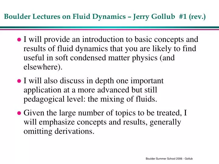
Boulder Lectures on Fluid Dynamics – Jerry Gollub #1 (rev.). I will provide an introduction to basic concepts and results of fluid dynamics that you are likely to find useful in soft condensed matter physics (and elsewhere).

E N D
Boulder Lectures on Fluid Dynamics – Jerry Gollub #1 (rev.) • I will provide an introduction to basic concepts and results of fluid dynamics that you are likely to find useful in soft condensed matter physics (and elsewhere). • I will also discuss in depth one important application at a more advanced but still pedagogical level: the mixing of fluids. • Given the large number of topics to be treated, I will emphasize concepts and results, generally omitting derivations.
Topics • Lecture 1 • Useful resources • Surface tension phenomena – an important static case • Basic fluid concepts: velocity field, etc. • Streaklines, pathlines, streamlines • Continuity; material derivative • Navier-Stokes equations; boundary conditions • Validity of the Navier-Stokes description • Lecture 2 • Reynolds number and other dimensionless parameters • Hydrodynamic similarity • Important steady flows: shear flow; tubes
Topics (continued) • Low Re flows: Stokes flow (LAST TOPIC IN THIS FILE) • Flow around particles • Drag on particles at low Re • Drag at higher Re • Sedimentation; particle interactions • Lubrication forces • Boundary layers • Lecture 3 • Vorticity and vortices • Surface waves • Convection phenomena • Pattern formation in Newtonian and polymeric fluids • Mixing - Introduction • Lecture 4 - Mixing of fluids; application to chemistry
Useful books on fluid dynamics • Multimedia Fluid Mechanics CD-Rom • B. Lautrup, Physics of Continuous Matter, 2005 • D.J. Tritton, Physical Fluid Dynamics, 1988 • I.M. Cohen and P.K. Kundu, Fluid Mechanics, 3rd edition (engineering orientation). • L.D Landau and E.M.Lifshitz, Fluid Mechanics (1987). • P.G. Drazin, Introduction to Hydrodynamic Stability (2002). • M.C.Cross and P. Hohenberg, Pattern Formation Out of Equilibrium, Reviews of Modern Physics (1993). • Flow of polymeric solutions, in M.P. Marder, Condensed Matter Physics, p. 378.
Surface Tension Phenomena - 1 • Increasing the area of an interface by dA requires work dW, analogous to mechanical work from volume changes: dW=dA (positive if dA>0) minimal areas are preferred. Typical values for : 72 mN/m H20. Equivalent to a force per unit length acting across a line within the surface. The pressure inside a droplet of radius a will be higher than outside due to surface tension: p=2/a . The pressure excess for a 1 cm soap bubble is only 30 Pa, but that for a 1 micron droplet or bacterium is about 3 atm. Physical origin of the surface energy: Energy of missing bonds for surface molecules.
Surface Tension Phenomena - 2 Q: Consider a very small bubble of air in a fluid container just below its lid. How small must the bubble be to be spherical? Hint: Consider the hydrostatic pressure difference across the bubble. Ans: about 3 mm. Capillary length • For non-spherical drops or bubbles, the pressure excess may be obtained from the principal radii of curvature: p=(1/R1 + 1/R2).
Surface Tension Phenomena - 3 • How does sap rise in plants? Evaporation from pores causes the water interface at the leaf pore (radius a) to be curved. The pressure in the water conduits (xylem) can be very negative, up to the point that p=2/a = gh, where is the water density, and h is the height. If a=1.5 microns, h can be 30 m, corresponding to negative pressures of 3 atm. Actual pores are as small as 20 nm 15 MPa. But why doesn’t it cavitate (nucleate vapor bubbles)? Nature423, 923 (26 June 2003) | doi: 10.1038/423923a, Plant hydraulics: The ascent of water, Melvin T. Tyree.
Surface Tension Phenomena - 4 • A cylindrical tube of fluid (e.g. from a faucet) of radius a is unstable to breakup. Why? Surface tension makes it contract, but this must occur at constant volume. It turns out that the area can be decreased at constant volume if the radius varies with a wavelength > 2a “Rayleigh-Plateau instability. • Key idea: Curvatures show that pressure is higher at a constriction than elsewhere if this condition is satisfied fluid moves away.
2a h Contact angles; capillary rise • Contact angles: When two fluids (e.g. a liquid and gas) meet at a solid surface, there is a characteristic contact angle that depends on the materials. Small for water/glass; obtuse for Hg on glass. • Leads to capillary rise in a tube of radius a. • Picture- Fishbones
Walking on fluid surfaces • See JWM Bush and DL Hu, Annu. Revs. Fluid Mech. 2006: “Walking on Water: Biolocomotion at the Interface”
Droplet genealogy: cascade of coalescences • The times shown are a–f, 0, 0.7, 1.8, 3.5, 5 and 50 ms, respectively, after first contact between the drop and pool. The drop acts as a lens, imaging a background square grid. (Images by S.Thoroddsen. and Yangfan Li., Nature 2006, vol. 2, p. 223)
Forces in fluids (or solids) • Stress tensor: Consider a small element of surface area treated as a vector (since orientation matters): dS = (dSx, dSy, dSz) The differential force acting across that surface can be written dF=dS, where is the stress tensor. Q: For a fluid that is not moving but has a pressure p, what is ? For a solid, or a moving fluid, it need not be diagonal, but it is symmetric, as first shown by Cauchy.
Velocity Field • Fluids can be treated as continua down to scales of about 20 Angstroms! The velocity field v(x,t) assigns a coarse-grained velocity to each fluid element that is currently at x. NOTE: Some books use u,v,w for the 3 components of v, instead ofvx, etc. Some also use u to mean v, whereas we have reserved u for the displacement field. Q:What would it be for a fluid that is uniformly rotating at angular velocity ? • Alternative Lagrangian description: Follow fluid elements starting at r for all subsequent times instead of giving v in fixed lab coordinates.
Streamlines, pathlines, streaklines • Streamlines, which are locally tangent to the velocity field, are solutions to this equation at a fixed time to: • If the velocity field is time-dependent, then the streamlines change, and tracer particles or dye spots need not follow them. They follow the current velocity field with initial condition xo : forming “pathlines” that solve • Yet a third way to describe a fluid flow is to release particles at a given starting position xo and initial time to, and ask what “streaklines” x(t, xo, to) they form at a given observation time t but various starting times to .
Streamlines, pathlines, streaklines (cont.) • Q: To test your understanding, suppose that v(x,t)=(a, bt, 0) and sketch the three types of lines I have just described: streamlines (at several times), pathlines from 0 to t, and streaklines from 0 to t. (Divide class into 3 groups.) • Movie: MMFM/kinematics/pathlines/steady and unsteady flows.
Continuity; material derivative • Continuity equation: • Incompressible flow: • Material time derivative: Q: What is the material derivative of the field x? Examples: narrowing tube; temperature field
Viscosity • Stress tensor in an isotropic moving fluid: • Careful: gradients are not just derivatives in non-cartesian coords. • Special case: Parallel shear flow • Viscosity – shear stress is linear in the velocity gradient or “strain rate”. • Water: =1 x 10⁻³ Pa s ; 1 centipoise in cgs units Kin.visc. / = = 1 x 10⁻⁶ m2/s (1 cS in cgs units) • For air: =1.8 x 10⁻⁵ Pa s; =1.5 x 10⁻⁵ m2/s Motions in air are more quickly damped.
Navier-Stokes equations • Navier-Stokes equation is obtained by setting the local density times acceleration equal to the effective force density: • Force density on a fluid element can be computed from gravity (or other external forces) and the stress tensor: (Use the def. of the stress tensor; compute forces across boundaries of a small box; and use Gauss’ theorem.)
Navier-Stokes equations (cont.) • Using the stress tensor for a Newtonian fluid leads to the Navier-Stokes equations (if incompressible): • Try writing out this equation for one component. • Note: 4 scalar equations for 4 fields • Q: Validity?
Validity of the Navier-Stokes equations • They describe motion on scales “much” larger than the molecular scale but much smaller than the system size. • The mean free path must be much less than the scale of interest. • If the fluid is not Newtonian, the relation between stress and strain rate must be specified: “Constitutive relation”. • Molecular dynamics calculations show that N-S works even on the few nm scale.
Boundary conditions • Generally, both normal and tangential components of velocity are zero at a solid surface. • No-slip usually works well down to a few nm scales, except in special cases (hydrophobic boundaries in microfluidics; dilute gasses). • Slip length: distance past a surface at which the velocity appears to extrapolate to zero (next slide) • Pressure is usually continuous across fluid boundaries (except for surface tension effects). • Q: What would happen at a gas/liquid boundary? (Movie: gas_fluid)
Evidence for slip at hydrophobic surfaces at high shear rates in microchannels • C-H Choi et al., Phys. Fluids 15, 2897 (2003)
Reynolds number (and other dimensionless parameters) • Ratio of advective (or inertial) to viscous terms in N-S: • Re for stirring coffee ~1000; for a bacterium in water, Re~ 10-5. • Many other dimensionless parameters arise; e.g. • Peclet number compares advection and diffusion.
Hydrodynamic similarity • If velocities, lengths, and pressures are made dimensionless using scales U,L, U2 , then the steady N-S equation looks like this: • The only parameter is Re. So steady flows at the same Re driven by geometrically similar boundaries will be identical when expressed non-dimensionally. • Works for time-dependent flows if U/L is used to make time dimensionless.
Simple shear flow • For a simple parallel shear flow (no gravity; no horizontal pressure gradient; no time dependence), N-S reduces to • Gives linear profile for a moving wall at y=d near a static one at y=0. • Wall shear stress in a fluid is very different from solid friction, which is large even at vanishing velocity. • Even better to use ball bearings so that there is no relative velocity.
Other steady flows: tubes and surfaces • Flow in a tube with pressure gradient G: Solve N-S in cylindrical coordinates for the speed and flux. • Entrance length: Momentum diffuses gradually; profile evolves. • Flow on an inclined surface at angle . Parabolic, but no gradient at the surface.
More on flow in tubes • The drag on a tube in the laminar regime can be found by taking the gradient of the velocity at the wall and multiplying by the area of the wall, to obtain D=8UL. • If Re is defined as Re=(2a)U/, then it is found that turbulence occurs around 2000-4000, but it can be much higher if perturbations are avoided. • In the turbulent regime, which does arise in arterial flow, the drag is augmented by a further factor f(Re) that grows slowly with Re, e.g. 7 at 10,000 and 20 at 100,000.
Stokes Flow- Low Re • Start from Navier-Stokes: • Look at steady solutions at low Re (“creeping flow”): • Movie of reversible stokes flow by G.I.Taylor