Download
1 / 15
150 likes | 302 Views
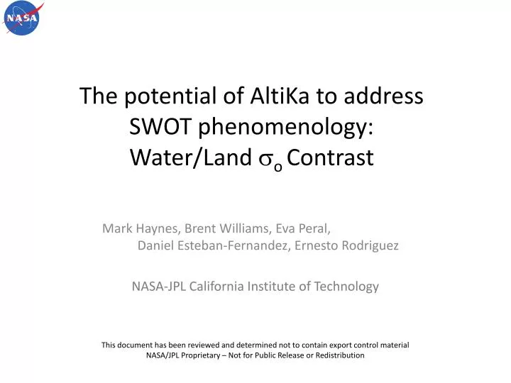
The potential of AltiKa to address SWOT phenomenology: Water/Land s o Contrast. Mark Haynes, Brent Williams, Eva Peral , Daniel Esteban- Fernandez , Ernesto Rodriguez NASA-JPL California Institute of Technology.

E N D
The potential of AltiKa to address SWOT phenomenology:Water/Land so Contrast Mark Haynes, Brent Williams, Eva Peral, Daniel Esteban-Fernandez, Ernesto Rodriguez NASA-JPL California Institute of Technology This document has been reviewed and determined not to contain export control material NASA/JPL Proprietary – Not for Public Release or Redistribution
Motivation • Normalized radar cross section: so • Characterizes the radar backscatter power of diffuse scattering scenes (ocean, trees, etc) • Depends on frequency, incidence angle, scattering statistics of scene • The ability of SWOT to distinguish land vs. water for hydrology depends heavily on the socontrast between land and water • Current sources for Ka-Band sovalues (ocean/land) • Difficult to model and measure • Few published measurements • JPL bridge measurements • AirSWOT will be a critical source • AltiKabenefits • Global Ka-band radar altimeter • Provides reflected power measurements • Same frequency, similar incidence angles as SWOT • AltiKa drawbacks • Nadir incidence produces bright returns from smooth water surfaces • Large footprint covers multiple land types • so angle dependence difficult to extract so so 30 meter range window 8 km swath Jet Propulsion Lab, CalTech
AltiKa Global Ocean Sigma0 Statistics • Histograms of AltiKa 1 Hz so data product • Orbit cycles {4, 5, 6} (1 cycle 1 month) • Upper bound ocean so for SWOT • AltiKa measures nadir incidence, so decreases with increasing observation angle Cycle 4: mean 11.8 dB, upper 68% cutoff = 10.1 dB Cycle 5: mean 11.8 dB, upper 68% cutoff = 10.1 dB Cycle 6: mean 11.6 dB, upper 68% cutoff = 10.1 dB • *Atmospheric correction included Jet Propulsion Lab, CalTech
Relative Water/Land Power Contrast • Initial approach: use AltiKa echoes as a basic reflected power measurement • Compare water/land integrated waveforms to obtain a relative comparison of reflected power • Hand picked water/land transitions with visually homogeneous vegetation without major bodies of water or irrigation • Caveats: nadir incidence, 30m range window over 8 km footprint Jet Propulsion Lab, CalTech
Case #1: Northwestern AustraliaCycle 6, Pass 34 Clean leading edges Signal above noise level Specular echo (tides, beach slope, estuary) Integrated waveform value plotted as antenna footprint 30 meter total range window at 0.3 meter resolution 4 dB ocean/land relative reflected power contrast Jet Propulsion Lab, CalTech
Case #1: Cycles 4 and 5, Pass 34 • Shows variability of water return echoes between cycles of the same scene • Dominated by first returns, not representative of higher incidence angles Cycle 4 Cycle 5 4 dB ocean/land contrast 10 dB ocean/land contrast Calm wind conditions Jet Propulsion Lab, CalTech
Case #2: West PapuaCycle 6, Pass 62 AltiKa’s nadir incidence angle and large footprint renders smooth water echoes unusable River crossing AltiKa 0o +/- 0.5o incidence SWOT 0.5o – 4.5o incidence Coastal water Inland forest Coastal forest River basin Ocean Mountain 6 dB contrast 10 dB contrast 4 dB contrast Jet Propulsion Lab, CalTech
Next steps: Quantitative inversion for land so • Use CNES and JPL simulation tools to invert for land so • Step 1) Altimeter waveform simulator • Goal: predict and confirm observed contrast levels and scattering phenomena, understand the sensitivity of the simulator to topography • CNES AltiKa Simulator • JPL SWOT Ocean Simulator • Step 2) Inversion algorithm • Inversion needed to separate topographic and incidence angle contributions to so • Approaches: a) Map echo power onto a DEM, b) in addition, iterate so map with the waveform simulation Jet Propulsion Lab, CalTech
AltiKa Waveform Simulation (CNES, JPL) Simulated • Case study #1 : Northwest Australia (Cycle 6, Pass 34) • Confirmation that land/sea contrast is ~5 dB • Input for CNES and JPL simulations • Ocean: s0 = 11 dB, Land: s0 = 6 dB, Beach: s0 = 45 dB • CNES: Lidar DEM • JPL: SRTM DEM • Run with simplified assumptions • Simulated returns highly sensitive to accuracy of DEM • Restricts areas of investigation to areas with good DEM • Variations of power with range can be simulated, can extrapolate to get angle variation in so Measured Simulated Jet Propulsion Lab, CalTech
Simulation of Beach (CNES) • Case study #1 : Northwest Australia (Cycle 6, Pass 34) • Focus on the bright return near the beach • Not permanent, not specific to Ka (alsoseen in Envisat data) • Seems to beexplained by a quasi specular return on a slightlyinclinedbeach • s0 = 45 dB, backscatterangular variation model = a gaussianwith FWHM = 0.25 deg Jet Propulsion Lab, CalTech
so Inversion from Measured Waveforms • Version 1 (non-iterative) • Project the power of each waveform and range line onto DEM, normalize by intersected area • Requires accurate DEM • Version 2 (iterative) • Use waveform simulator to model returns • Parameterize angle dependence of so • Also requires land type classification and accurate DEM Power projection onto DEM Same pixels are seen from multiple sensor positions Inversion separates the contribution of each pixel to different waveforms Jet Propulsion Lab, CalTech
Viable Global Land Echoes for so Statistics dB (power) • Ultimate goal is to obtain global statistics of land so at Ka band and 0.5o-4.5o incidence angles • Want to use AltiKa to provide SWOT with an upper bound • AltiKa not designed to work over land (30 m range window) • Anywhere the return is above the noise can potentially be used as a power measurement • Look for integrated land echo powers above the noise • Low SNR: extreme topography (mountains), diffuse scattering • Good SNR: Altimeter was tracking Noise level = 51 dB 5, 10, 15 dB minimum SNR 50% global land surface potentially available for land so statistics Noise level = 51 dB Jet Propulsion Lab, CalTech
Viable Global Ice Echoes for so Statistics • AltiKa has numerous ice so products (have not yet looked at these in detail) • Same integrated waveform analysis as land (previous slide) • Segmented with ‘ice_flag’ • 80% of integrated ice returns 10 dB above noise • Useful for hydrology in frozen conditions Noise level = 51 dB 5, 10, 15 dB minimum SNR Noise level = 51 dB 80% of ice surface potentially available for ice so statistics Jet Propulsion Lab, CalTech
Conclusions • Initial evaluation of AltiKa to address SWOT phenomenology • AltiKais a valuable data set for SWOT (global, similar system parameters) • Excellent ocean so statistics • Reasonable relative ocean/land contrast • Early evaluation is promising, more information to extract • Issues using AltiKa for SWOT evaluation • Nadir incidence and limited range window • Scope of next steps: • Refine waveform simulators (CNES, JPL), update DEMs (SRTM 30m) • Formal inversion for so with complete models • Investigate ground truth (US National Land Classification Data) • Automate site selection for global sampling • Schedule of next steps • In the next 2-3 months, determine if we can extract hard values for land so as a function of incidence angle with global sampling • Design AirSWOT campaigns to cross validate these efforts (already have AirSWOT flights under AltiKa lines) Jet Propulsion Lab, CalTech
AltiKa Geometry Area projection for 65 range bins Incidence angle taken at leading edge of bin Assume, flat surface h = 787 km (for ocean waveforms on previous slide) Areas are nearly the same qi h + nDr 0.4 deg incidence h a Dr Jet Propulsion Lab, CalTech