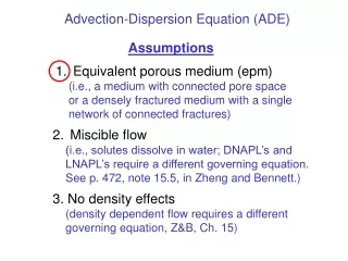
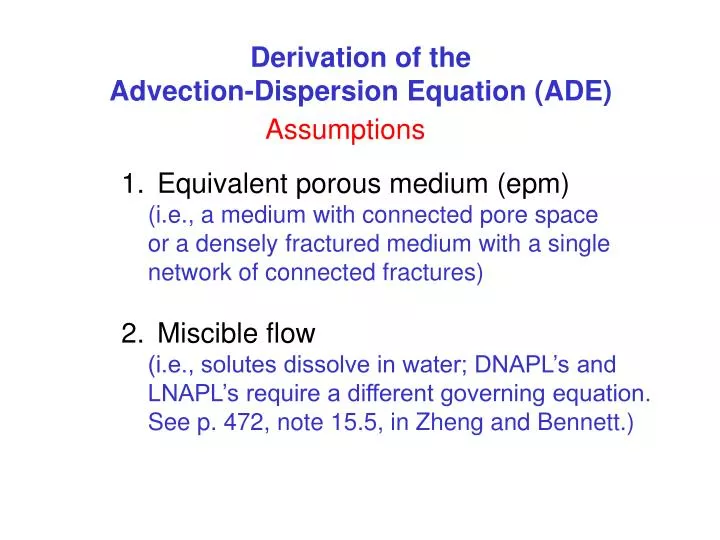
Derivation of the Advection-Dispersion Equation (ADE)

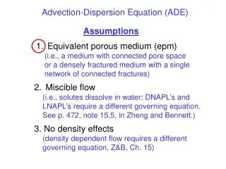
1. Derivation of the Advection-Dispersion Equation (ADE) Assumptions • Equivalent porous medium (epm) • (i.e., a medium with connected pore space • or a densely fractured medium with a single • network of connected fractures) • Miscible flow • (i.e., solutes dissolve in water; DNAPL’s and • LNAPL’s require a different governing equation. • See p. 472, note 15.5, in Zheng and Bennett.)

2. 3. No density effects Density-dependent flowrequires a different governing equation. See Zheng and Bennett, Chapter 15. Figures from Freeze & Cherry (1979)

3. Derivation of the Advection-Dispersion Equation (ADE) Darcy’s law: h1 h1 h2 h2 q = Q/A advective flux fA = q c s s f = F/A

4. How about Fick’s law of diffusion? where Dd is the effective diffusion coefficient. How do we quantify the dispersive flux? h1 fA = advective flux = qc f = fA + fD h2 s

5. Dual Porosity Domain Figure from Freeze & Cherry (1979) Fick’s law describes diffusion of ions on a molecular scale as ions diffuse from areas of higher to lower concentrations.

6. We need to introduce a “law” to describe dispersion, to account for the deviation of velocities from the average linear velocity calculated by Darcy’s law. Average linear velocity True velocities

7. porosity where D is the dispersion coefficient. We will assume that dispersion follows Fick’s law, or in other words, that dispersion is “Fickian”. This is an important assumption; it turns out that the Fickian assumption is not strictly valid near the source of the contaminant.

8. Porosity () Later we will define the dispersion coefficient in terms of v and therefore we insert  now: Mathematically, porosity functions as a kind of units conversion factor. for example: q c = v  c

9. Assume 1D flow qx s Case 1 and a line source

10. Assume 1D flow qx s D is the dispersion coefficient. It includes the effects of dispersion and diffusion. Dx is sometimes written DL and called the longitudinal dispersion coefficient. Case 1 porosity Advective flux Dispersive flux

11. Assume 1D flow qx s Case 2 and a point source

12. Dispersive fluxes fA = qxc Advective flux Dx represents longitudinal dispersion (& diffusion); Dy represents horizontal transverse dispersion (& diffusion); Dz represents vertical transverse dispersion (& diffusion).

13. Continuous point source Average linear velocity Instantaneous point source center of mass Figure from Freeze & Cherry (1979)

14. longitudinal dispersion transverse dispersion Instantaneous Point Source Gaussian Figure from Wang and Anderson (1982)

15. Derivation of the ADE for 1D uniform flow and 3D dispersion (e.g., a point source in a uniform flow field) vx = a constant vy = vz = 0 f = fA + fD Mass Balance: Flux out – Flux in = change in mass

16. Porosity () In practice, we assume that total porosity equals effective porosity for purposes of deriving the advection-dispersion eqn. See Zheng and Bennett, pp. 56-57. There are two types of porosity in transport problems: total porosity and effective porosity. Total porosity includes immobile pore water, which contains solute and therefore it should be accounted for when determining the total mass in the system. Effective porosity accounts for water in interconnected pore space, which is flowing/mobile.

17. Definition of the Dispersion Coefficient in a 1D uniform flow field Dx = xvx + Dd Dy = yvx + Dd Dz = zvx + Dd vx = a constant vy = vz = 0 where x y z are known as dispersivities. Dispersivity is essentially a “fudge factor” to account for the deviations of the true velocities from the average linear velocities calculated from Darcy’s law. Rule of thumb:y= 0.1x ;z = 0.1y

18. ADE for 1D uniform flow and 3D dispersion No sink/source term; no chemical reactions Question: If there is no source term, how does the contaminant enter the system?

19. Simpler form of the ADE Uniform 1D flow; longitudinal dispersion; No sink/source term; no chemical reactions Question: Is this equation valid for both point and line sources? There is a famous analytical solution to this form of the ADE with a continuous line source boundary condition. The solution is called the Ogata & Banks solution.

20. Effects of dispersion on the concentration profile no dispersion dispersion t4 t1 t2 t3 (Freeze & Cherry, 1979, Fig. 9.1) (Zheng & Bennett, Fig. 3.11)

21. Effects of dispersion on the breakthrough curve

22. Instantaneous Point Source Gaussian Figure from Wang and Anderson (1982)

23. Breakthrough curve long tail Concentration profile

24. Microscopic or local scale dispersion Figure from Freeze & Cherry (1979)

25. Macroscopic Dispersion (caused by the presence of heterogeneities) Homogeneous aquifer Heterogeneous aquifers Figure from Freeze & Cherry (1979)

26. Dispersivity () is a measure of the heterogeneity present in the aquifer. A very heterogeneous porous medium has a higher dispersivity than a slightly heterogeneous porous medium.

27. Dispersion in a 3D flow field

28. global local z z’ x’  x Kxx Kxy Kxz Kyx Kyy Kyz Kzx Kzy Kzz K’x 0 0 0 K’y 0 0 0 K’z K = [K] = [R]-1 [K’] [R]

30. Dxx Dxy Dxz Dyx Dyy Dyz Dzx Dzy Dzz D = In general: D >> Dd Dispersion Coefficient (D) D = D + Dd D represents dispersion Dd represents molecular diffusion

32. Dx = xvx + Dd Dy = yvx + Dd Dz = zvx + Dd Recall, that for 1D uniform flow: In a 3D flow field it is not possible to simplify the dispersion tensor to three principal components. In a 3D flow field, we must consider all 9 components of the dispersion tensor. The definition of the dispersion coefficient is more complicated for 2D or 3D flow. See Zheng and Bennett, eqns. 3.37-3.42.

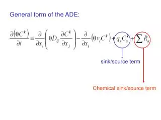
33. General form of the ADE: Expands to 9 terms Expands to 3 terms (See eqn. 3.48 in Z&B)