Download
1 / 1
10 likes | 113 Views
Large Eddy Simulations of Entrainment and Inversion Structure. Alison Fowler (MRes Physics of Earth and Atmosphere) Supervisor: Ian Brooks. Statistics of the Entrainment Zone.

E N D
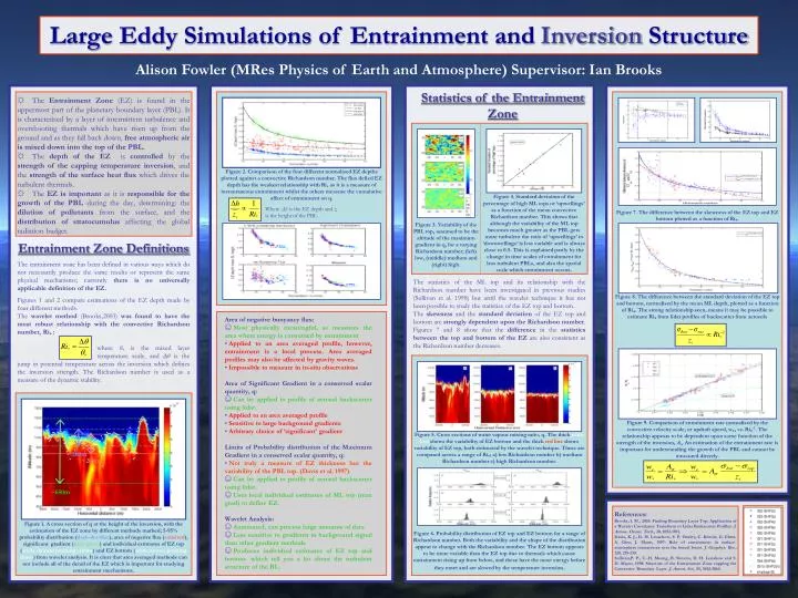
Large Eddy Simulations of Entrainment and Inversion Structure Alison Fowler(MRes Physics of Earth and Atmosphere) Supervisor: Ian Brooks Statistics of the Entrainment Zone • The Entrainment Zone (EZ) is found in the uppermost part of the planetary boundary layer (PBL). It is characterised by a layer of intermittent turbulence and overshooting thermals which have risen up from the ground and as they fall back down, free atmospheric air is mixed down into the top of the PBL. • The depth of the EZ is controlled by the strength of the capping temperature inversion, and the strength of the surface heat flux which drives the turbulent thermals. • The EZ is important as it is responsible for the growth of the PBL during the day, determining: the dilution of pollutants from the surface, and the distribution of stratocumulus affecting the global radiation budget. Figure 2. Comparison of the four different normalised EZ depths plotted against a convective Richardson number. The flux defied EZ depth has the weakest relationship with Ri* as it is a measure of instantaneous entrainment whilst the others measure the cumulative affect of entrainment on q. Figure 4. Standard deviation of the percentage of high ML tops or ‘upwellings’ as a function of the mean convective Richardson number. This shows that although the variability of the ML top becomes much greater as the PBL gets more turbulent the ratio of ‘upwellings’ to ‘downwellings’ is less variable and is always close to 0.5. This is explained partly by the change in time scales of entrainment for less turbulent PBLs, and also the spatial scale which entrainment occurs. Where Δh is the EZ depth and zi is the height of the PBL. Figure 7. The difference between the skewness of the EZ top and EZ bottom plotted as a function of Ri*. Figure 3. Variability of the PBL top, assumed to be the altitude of the maximum gradient in q, for a varying Richardson number; (left) low, (middle) medium and (right) high. Entrainment Zone Definitions The entrainment zone has been defined in various ways which do not necessarily produce the same results or represent the same physical mechanisms; currently there is no universally applicable definition of the EZ. Figures 1 and 2 compare estimations of the EZ depth made by four different methods. The wavelet method (Brooks,2003) was found to have the most robust relationship with the convective Richardson number, Ri* : where θ*is the mixed layer temperature scale, and Δθ is the jump in potential temperature across the inversion which defines the inversion strength. The Richardson number is used as a measure of the dynamic stability. The statistics of the ML top and its relationship with the Richardson number have been investigated in previous studies (Sullivan et al. 1998) but until the wavelet technique it has not been possible to study the statistics of the EZ top and bottom. The skewness and the standard deviation of the EZ top and bottom are strongly dependent upon the Richardson number. Figures 7 and 8 show that the difference in the statistics between the top and bottom of the EZ are also consistent as the Richardson number decreases. Figure 8. The difference between the standard deviation of the EZ top and bottom, normalised by the mean ML depth, plotted as a function of Ri*. The strong relationship seen, means it may be possible to estimate Ri* from lidar profiles of backscatter from aerosols • Area of negative buoyancy flux: • Most physically meaningful, as measures the area where energy is consumed by entrainment • Applied to an area averaged profile, however, entrainment is a local process. Area averaged profiles may also be affected by gravity waves. • Impossible to measure in in-situ observations • Area of Significant Gradient in a conserved scalar quantity, q: • Can be applied to profile of aerosol backscatter using lidar. • Applied to an area averaged profile • Sensitive to large background gradients • Arbitrary choice of ‘significant’ gradient • Limits of Probability distribution of the Maximum Gradient in a conserved scalar quantity, q: • Not truly a measure of EZ thickness but the variability of the PBL top. (Davis et al. 1997) • Can be applied to profile of aerosol backscatter using lidar. • Uses local individual estimates of ML top (max grad) to define EZ. • Wavelet Analysis: • Automated, can process large amounts of data • Less sensitive to gradients in background signal than other gradient methods • Produces individual estimates of EZ top and bottom- which tell you a lot about the turbulent structure of the BL. Figure 9. Comparison of entrainment rate normalised by the convective velocity scale, or updraft speed, w*, vs. Ri*-1. The relationship appears to be dependent upon some function of the strength of the inversion, Aσ. An estimation of the entrainment rate is important for understanding the growth of the PBL and cannot be measured directly. Figure 5. Cross sections of water vapour mixing ratio, q. The thick white line shows the variability of EZ bottom and the thick red line shows variability of EZ top, both estimated by the wavelet technique. These are compared across a range of Ri*; a) low Richardson number b) medium Richardson number c) high Richardson number. ~200m ~200m ~650m References: Brooks, I. M., 2003: Finding Boundary Layer Top: Application of a Wavelet Covariance Transform to Lidar Backscatter Profiles. J. Atmos. Ocean. Tech., 20, 1092-1105. Davis, K. J., D. H. Lenschow, S. P. Oncley, C. Kiemle, G. Ehret, A. Giez, J. Mann, 1997: Role of entrainment in surface-atmosphere interactions over the boreal forest. J. Geophys. Res., 120, 219-230. Sullivan,P. P., C.-H. Moeng, B. Stevens, D. H. Lenshow and S. D. Mayor, 1998: Structure of the Entrainment Zone capping the Convective Boundary Layer. J. Atmos. Sci., 55, 3042-3064. Figure 1. A cross section of q at the height of the inversion, with the estimation of the EZ zone by different methods marked; 5-95% probability distribution (dash-dot blue), area of negative flux (solid red), significant gradient (dash green) and individual estimates of EZ top (white upward pointing arrows) and EZ bottom (white arrows pointing down) from wavelet analysis. It is clear that area averaged methods can not include all of the detail of the EZ which is important for studying entrainment mechanisms. Figure 6. Probability distribution of EZ top and EZ bottom for a range of Richardson number. Both the variability and the shape of the distribution appear to change with the Richardson number. The EZ bottom appears to be more variable than the EZ top due to thermals which cause entrainment rising up from below, and these have the most energy before they enter and are slowed by the temperature inversion.