Download

1 / 49
490 likes | 762 Views
Heaps. Heaps. A heap is a data structure similar to a binary search tree. However, heaps are not sorted as binary search trees are. And, heaps are always complete binary trees (only vacancies are at the bottom level , and to the right ).

E N D
Heaps • A heap is a data structure similar to a binary search tree. • However, heaps are not sorted as binary search trees are. • And, heaps are always complete binary trees (only vacancies are at the bottom level, and to the right). • Therefore, we always know what the maximum size of a heap is.
Heaps • Unlike a binary search tree, the value of each node in a heap is greater than or equal to the value in each of its children. • In addition, there is no relationship between the values of the children; you don't know which child contains the larger value. • Heaps are used to implement priority queues.
Heaps When a complete binary tree is built, its first node must be the root. Root A heap is a certain kind of complete binary tree.
Heaps The second node is always the left child of the root. Complete binary tree. Left child of the root
Heaps The third node is always the right child of the root. Complete binary tree. Right child of the root
Heaps The next nodes always fill the next level from left-to-right. Complete binary tree.
Heaps The next nodes always fill the next level from left-to-right. Complete binary tree.
Heaps The next nodes always fill the next level from left-to-right. Complete binary tree.
Heaps The next nodes always fill the next level from left-to-right. Complete binary tree.
Heaps Complete binary tree.
Heaps 45 35 23 27 21 22 4 19 Each node in a heap contains a key that can be compared to other nodes' keys. A heap is a certain kind of complete binary tree.
Heaps 45 35 23 27 21 22 4 19 The "heap property" requires that each node's key is >= the keys of its children A heap is a certain kind of complete binary tree.
Adding a Node to a Heap 45 35 23 27 21 22 4 19 42 • Put the new node in the next available spot. • Push the new node upward, swapping with its parent until the new node reaches an acceptable location.
45 35 23 42 21 22 4 19 27 Adding a Node to a Heap • Put the new node in the next available spot. • Push the new node upward, swapping with its parent until the new node reaches an acceptable location.
Adding a Node to a Heap 45 42 23 35 21 22 4 19 27 • Put the new node in the next available spot. • Push the new node upward, swapping with its parent until the new node reaches an acceptable location.
Adding a Node to a Heap 45 42 23 35 21 22 4 19 27 • The parent has a key that is >= new node, or • The node reaches the root. • The process of pushing the new node upward is called reheapificationupward.
Removing the Top of a Heap 45 42 23 35 21 22 4 19 27 • Move the last node onto the root.
Removing the Top of a Heap 27 42 23 35 21 22 4 19 • Move the last node onto the root.
Removing the Top of a Heap 27 42 23 35 21 22 4 19 • Move the last node onto the root. • Push the out-of-place node downward, swapping with its larger child until the new node reaches an acceptable location.
Removing the Top of a Heap 42 27 23 35 21 22 4 19 • Move the last node onto the root. • Push the out-of-place node downward, swapping with its larger child until the new node reaches an acceptable location. • When we push a node downward it is important to swap it with its largest child.
Removing the Top of a Heap 42 35 23 27 21 22 4 19 • Move the last node onto the root. • Push the out-of-place node downward, swapping with its larger child until the new node reaches an acceptable location.
Removing the Top of a Heap 42 35 23 27 21 22 4 19 • The children all have keys <= the out-of-place node, or • The node reaches the leaf. • The process of pushing the new node downward is called reheapificationdownward.
Implementing a Heap: Array • Operations on Heaps are best visualized in the tree form, but the heap doesn't have to be implemented as a linked structure. • The regularity of its shape makes it possible to encode the parent/children pointers implicitly as array locations.
Implementing a Heap 42 35 23 27 21 • We will store the data from the nodes in a partially-filled array. An array of data
Implementing a Heap 42 35 23 27 21 • Data from the root goes in thefirst location of the array. 42 An array of data
Implementing a Heap 42 35 23 27 21 • Data from the next row goesin the next two array locations. 42 35 23 An array of data
Implementing a Heap 42 35 23 27 21 • Data from the next row goesin the next two array locations. 42 35 23 27 21 An array of data
Implementing a Heap 42 35 23 27 21 • Data from the next row goesin the next two array locations. 42 35 23 27 21 An array of data We don't care what's in this part of the array.
Important Points about the Implementation 42 35 23 27 21 • The links between the tree's nodes are not actually stored as pointers, or in any other way. • The only way we "know" that "the array is a tree" is from the way we manipulate the data. 42 35 23 27 21 An array of data
Important Points about the Implementation 42 35 23 27 21 • If you know the index of a node, then it is easy to figure out the indexes of that node's parent and children. Formulas are given in the book. 42 35 23 27 21 [1] [2] [3] [4] [5]
Summary • A heap is a complete binary tree, where the entry at each node is greater than or equal to the entries in its children. • To add an entry to a heap, place the new entry at the next available spot, and perform a reheapification upward. • To remove the biggest entry, move the last node onto the root, and perform a reheapification downward.
Priority Queues • In multi-user environments, a scheduler decides which of many available jobs to run at any time, when to switch to next etc. • Think of computer systems, routers, printers etc.. Often, schedulers use a simple FIFO queue. This can be particularly bad if there is wide disparity in job sizes: • 1-page vs. 100 page print job; • 48 byte vs. 8K byte packet; • telnet commands vs. big ftp • A more refined form of the queue is called Priority Queue, in which jobs can be assigned priorities, and the queue pulls jobs out based on their priority.
Priority Queues & Heaps • A priority queue is an Abstract Data Type! • Which, can be implemented using heaps. Think of a To-Do lists; each item has a priority value which reflects the urgency with which each item needed to be addressed • Priority Queue ADT allows at least the following 2 operations: a. Insert an element; the key is the priority; b. DeleteMin; remove the element with the smallest key. • (Think of priority as being the rank; smallest key is the most urgent job.)
Priority Queues & Heaps • By preparing a priority queue, we can determine which item is the next highest priority. • A priority queue maintains items sorted in descending order of their priority value -- so that the item with the highest priority value is always at the beginning of the list.
Priority Queues & Heaps • Priority Queue ADT operations can be implemented using heaps... • which is a weaker binary tree but sufficient for the efficient performance of priority queue operations. • Let's look at a heap:
Priority Queues & Heaps • To remove an item from a heap, we remove the largest item (or the item with the highest priority). • Because the value of every node is greater than or equal to that of either of its children, the largest value must be the root of the tree. • A remove operation is simply to remove the item at the root and return it to the calling routine.
Priority Queues & Heaps • Once you have removed the largest value, you are left with two disjoint heaps: • Therefore, you need to transform the nodes • Move the last node and place it in the root • Then take that value and trickle it down the tree until it reaches a node in which it will not be out of place.
Priority Queues & Heaps • To insert an item, we use just the opposite strategy. • We insert at the bottom of the tree and trickle the number upward to be in the proper place. • With insert, the number of swaps cannot exceed the height of the tree -- so that is the worst case!
Priority Queues & Heaps • The real advantage of a heap is that it is always balanced. • It makes a heap more efficient for implementing a priority queue than a binary search tree because the operations that keep a binary search tree balanced are far more complex than the heap operations. • However, heaps are not useful if you want to try to traverse a heap in sorted order -- or retrieve a particular item.
Heapsort • A heapsort uses a heap to sort a list of items that are not in any particular order. • The first step of the algorithm transforms the array into a heap. • We do this by inserting the numbers into the heap and having them trickle up...one number at a time.
Heapsort • A better approach is to put all of the numbers in a binary tree -- in the order you received them. • Then, perform the algorithm we used to adjust the heap after deleting an item. • This will cause the smaller numbers to trickle down to the bottom.
Assignment Create a program that uses a binary tree Create a program that uses a heap for a priority queue
std::priority_queue The STL has a Priority Queue: std::priority_queue, in <queue>. • STL documentation does not call std::priority_queuea “container”, but rather a “container adapter”. • This is because std::priority_queueis explicitly a wrapper around some other container. You get to pick what that container is. • You say “std::priority_queue<T, container<T> >”. “T” is the value type. “container” can be std::vector or std::deque. “container<T>” can be any standard-conforming random-access sequence container. • container defaults to std::vector. You can say just “std::priority_queue<T>” to get “std::priority_queue<T, std::vector<T> >”.
std::priority_queue The member function names used by std::priority_queueare the same as those used by std::stack. • Not those used by std::queue. • Thus, std::priority_queuehas “top”, not “front”. Given a variable pqof type std::priority_queue<T>, you can do: • pq.top() • pq.push(item) “item” is some value of type T. • pq.pop() • pq.empty() • pq.size()