Download
1 / 23
240 likes | 254 Views
On the computation of the defining polynomial of the algebraic Riccati equation. Yamaguchi Univ. Takuya Kitamoto Cybernet Systems, Co. LTD Tetsu Yamaguchi. Outline of the presentation. What is ARE (Algebraic Riccati Equation)? Properties of ARE Problem formulation Algorithm description

E N D
On the computation of the defining polynomial of the algebraic Riccati equation Yamaguchi Univ. Takuya Kitamoto Cybernet Systems, Co. LTD Tetsu Yamaguchi
Outline of the presentation • What is ARE (Algebraic Riccati Equation)? • Properties of ARE • Problem formulation • Algorithm description • Numerical experiments • Conclusion
Important equation for control theory (H2 optimal control, etc) Symmetric solutions (solution matrices are symmetric) are important. There are 2^n symmetric solutions. When matrices A, W, Q are numerical matrices, a numerical algorithm to compute the solutions is already known. The numerical algorithm can not be applied when matrices A, W, Q contain a parameter. Properties of ARE
Problem formulation Example:
We can compute the defining polynomial of entries of P, not P itself.
The method with Groebner Basis: Effective for only small degree n (n=2), because of its heavy numerical complexities
Conversion from floating point numbers to integers • Arbitrary precision arithmetic can be used. • Precision required is unknown.
Conversion from integers to polynomials • Polynomial interpolation can be used. • The degree of the polynomial is unknown.
Numerical experiments (2) Environments: Maple 10 on the machine with Pentium M 2.0GHz, 1.5Gbyte memory Computation time (in seconds)
Conclusion • An algorithm to compute the defining polynomial of ARE with a parameter is given. • The algorithm uses polynomial interpolations and arbitrary precision arithmetic. • Numerical experiments suggest that the algorithm is practical for the system with size n<5. • The algorithm is suitable for multi-CPU environments.
Future direction • Further improvements of efficiency is necessary. • Modular algorithm instead of floating point arithmetic can be used (provided the head coefficient is known). • Extend application of the defining polynomial.