Download
1 / 144
1.46k likes | 1.52k Views
Optimization. Nonlinear programming: One dimensional minimization methods. Introduction. The basic philosophy of most of the numerical methods of optimization is to produce a sequence of improved approximations to the optimum according to the following scheme:

E N D
Optimization Nonlinear programming: One dimensional minimization methods
Introduction The basic philosophy of most of the numerical methods of optimization is to produce a sequence of improved approximations to the optimum according to the following scheme: • Start with an initial trial point Xi • Find a suitable direction Si(i=1 to start with) which points in the general direction of the optimum • Find an appropriate step length i* for movement along the direction Si • Obtain the new approximation Xi+1as • Test whether Xi+1is optimum. If Xi+1is optimum, stop the procedure. Otherwise set a new i=i+1 and repeat step (2) onward.
Introduction • The iterative procedure indicated is valid for unconstrained as well as constrained optimization problems. • If f(X) is the objective function to be minimized, the problem of determining i* reduces to finding the value i = i* that minimizes f (Xi+1) = f (Xi+ i Si) = f (i ) for fixed values of Xi and Si. • Since f becomes a function of one variable i only, the methods of finding i* in the previous slide are called one-dimensional minimization methods.
One dimensional minimization methods • Analytical methods (differential calculus methods) • Numerical methods • Elimination methods • Unrestricted search • Exhaustive search • Dichotomous search • Fibonacci method • Golden section method • Interpolation methods • Requiring no derivatives (quadratic) • Requiring derivatives • Cubic • Direct root • Newton • Quasi-Newton • Secant
One dimensional minimization methods Differential calculus methods: • Analytical method • Applicable to continuous, twice differentiable functions • Calculation of the numerical value of the objective function is virtually the last step of the process • The optimal value of the objective function is calculated after determining the optimal values of the decision variables
One dimensional minimization methods Numerical methods: • The values of the objective function are first found at various combinations of the decision variables • Conclusions are then drawn regarding the optimal solution • Elimination methods can be used for the minimization of even discontinuous functions • The quadratic and cubic interpolation methods involve polynomial approximations to the given function • The direct root methods are root finding methods that can be considered to be equivalent to quadratic interpolation
Unimodal function • A unimodal function is one that has only one peak (maximum) or valley (minimum) in a given interval • Thus a function of one variable is said to be unimodal if, given that two values of the variable are on the same side of the optimum, the one nearer the optimum gives the better functional value (i.e., the smaller value in the case of a minimization problem). This can be stated mathematically as follows: A function f (x) is unimodal if • x1 < x2 < x* implies that f (x2) < f (x1)and • x2 > x1 > x* implies that f (x1) < f (x2)where x* is the minimum point
Unimodal function • Examples of unimodal functions: • Thus, a unimodal function can be a nondifferentiable or even a discontinuous function • If a function is known to be unimodal in a given range, the interval in which the minimum lies can be narrowed down provided that the function values are known at two different values in the range.
Unimodal function • For example, consider the normalized interval [0,1] and two function evaluations within the interval as shown: • There are three possible outcomes: • f1 <f2 • f1 >f2 • f1 =f2
Unimodal function • If the outcome is f1 <f2, the minimizing x can not lie to the rightof x2 • Thus, that part of the interval [x2,1]can be discarded and a new small interval of uncertainty,[0, x2]results as shown in the figure
Unimodal function • If the outcome is f (x1)>f (x2), the interval [0, x1] can bediscarded to obtain a new smaller interval of uncertainty,[x1, 1].
Unimodal function • If f1 =f2 , intervals [0, x1] and [x2,1] can both be discarded to obtain the new interval of uncertainty as [x1,x2]
Unimodal function • Furthermore, if one of the experiments (function evaluations in the elimination method) remains within the new interval, as will be the situation in Figs (a) and (b), only one other experiment need be placed within the new interval in order that the process be repeated. • In Fig (c), two more experiments are to be placed in the new interval in order to find a reduced interval of uncertainty.
Unimodal function • The assumption of unimodality is made in all the elimination techniques • If a functionis known to be multimodal (i.e., having several valleys or peaks), the range of the function can be subdivided into several parts and the function treated as a unimodal function in each part.
Elimination methods In most practical problems, the optimum solution is known to lie within restricted ranges of the design variables. In some cases, this range is not known, and hence the search has to be made with no restrictions on the values of the variables. UNRESTRICTED SEARCH • Search with fixed step size • Search with accelerated step size
Unrestricted Search Search with fixed step size • The most elementary approach for such a problem is to use a fixed step size and move from an initial guess point in a favorable direction (positive or negative). • The step size used must be small in relation to the final accuracy desired. • Simple to implement • Not efficient in many cases
Unrestricted Search Search with fixed step size • Start with an initial guess point, say, x1 • Find f1 = f (x1) • Assuming a step size s, find x2=x1+s • Find f2 = f (x2) • If f2 < f1, and if the problem is one of minimization, the assumption of unimodality indicates that the desired minimum can not lie at x < x1. Hence the search can be continued further along points x3, x4,….using the unimodality assumption while testing each pair of experiments. This procedure is continued until a point, xi=x1+(i-1)s, shows an increase in the function value.
Unrestricted Search Search with fixed step size (cont’d) • The search is terminated at xi, and either xi or xi-1can be taken as the optimum point • Originally, if f1 < f2 , the search should be carried in the reverse direction at points x-2, x-3,….,where x-j=x1- ( j-1 )s • If f2=f1 , the desired minimum lies in between x1and x2, and the minimum point can be taken as either x1or x2. • If it happens that both f2and f-2are greater than f1, it implies that the desired minimum will lie in the double interval x-2 < x < x2
Unrestricted Search Search with accelerated step size • Although the search with a fixed step size appears to be very simple, its major limitation comes because of the unrestricted nature of the region in which the minimum can lie. • For example, if the minimum point for a particular function happens to be xopt=50,000and in the absence of knowledge about the location of the minimum, if x1and s are chosen as 0.0 and 0.1, respectively, we have to evaluate the function 5,000,001 times to find the minimum point. This involves a large amount of computational work.
Unrestricted Search Search with accelerated step size (cont’d) • An obvious improvement can be achieved by increasing the step size gradually until the minimum point is bracketed. • A simple method consists of doubling the step size as long as the move results in an improvement of the objective function. • One possibility is to reduce the step length after bracketing the optimum in ( xi-1, xi). By starting either from xi-1 or xi, the basic procedure can be applied with a reduced step size. This procedure can be repeated until the bracketed interval becomes sufficiently small.
Example Find the minimum of f = x (x-1.5)by starting from 0.0 with an initial step size of 0.05. Solution: The function value at x1 is f1=0.0. If we try to start moving in the negative x direction, we find that x-2=-0.05and f-2=0.0775. Since f-2>f1, the assumption of unimodality indicates that the minimum can not lie toward the left of x-2. Thus, we start moving in the positive x direction and obtain the following results:
Example Solution: From these results, the optimum point can be seen to be xopt x6=0.8. In this case, the points x6and x7do not really bracket the minimum point but provide information about it. If a better approximation to the minimum is desired, the procedure can be restarted from x5with a smaller step size.
Exhaustive search • The exhaustive search method can be used to solve problems where the interval in which the optimum is known to lie is finite. • Let xs and xf denote, respectively, the starting and final points of the interval of uncertainty. • The exhaustive search method consists of evaluating the objective function at a predetermined number of equally spaced points in the interval (xs, xf), and reducing the interval of uncertainty using the assumption of unimodality.
Exhaustive search • Suppose that a function is defined on the interval (xs, xf), and let it be evaluated at eight equally spaced interior points x1 to x8. The function value appears as: • Thus, the minimum must lie, according to the assumption of unimodality, between points x5 and x7. Thus the interval (x5,x7) can be considered as the final interval of uncertainty.
Exhaustive search • In general, if the function is evaluated at n equally spaced points in the original interval of uncertainty of length L0= xf - xs, and if theoptimum value of the function (among the n function values) turns out to be at point xj, the final interval of uncertainty is given by: • The final interval of uncertainty obtainable for different number of trials in the exhaustive search method is given below:
Exhaustive search • Since the function is evaluated at all n points simultaneously, this method can be called a simultaneous search method. • This method is relatively inefficient compared to the sequential search methods discussed next, where the information gained from the initial trials is used in placing the subsequent experiments.
Example Find the minimum of f = x(x-1.5) in the interval (0.0,1.0) to within 10 % of the exact value. Solution: If the middle point of the final interval of uncertainty is taken as the approximate optimum point, the maximum deviation could be 1/(n+1) times the initial interval of uncertainty. Thus, to find the optimum within 10% of the exact value, we should have
Example By taking n = 9, the following function values can be calculated: Since f7 = f8 , the assumption of unimodality gives the final interval ofuncertainty as L9= (0.7,0.8). By taking the middle point of L9(i.e.,0.75) as an approximation to the optimum point, we find that it is in fact, the true optimum point.
Dichotomous search • The exhaustive search method is a simultaneous search method in which all the experiments are conducted before any judgement is made regarding the location of the optimum point. • The dichotomous search method , as well as the Fibonacci and the golden section methods discussed in subsequent sections, are sequential search methods in which the result of any experiment influences the location of the subsequent experiment. • In the dichotomous search, two experiments are placed as close as possible at the center of the interval of uncertainty. • Based on the relative values of the objective function at the two points, almost half of the interval of uncertainty is eliminated.
Dichotomous search • Let the positions of the two experiments be given by: where is a small positive number chosen such that the two experiments give significantly different results.
Dichotomous Search • Then the new interval of uncertainty is given by (L0/2+/2). • The building block of dichotomous search consists of conducting a pair of experiments at the center of the current interval of uncertainty. • The next pair of experiments is, therefore, conducted at the center of the remaining interval of uncertainty. • This results in the reduction of the interval of uncertainty by nearly a factor of two.
Dichotomous Search • The intervals of uncertainty at the ends of different pairs of experiments are given in the following table. • In general, the final interval of uncertainty after conducting n experiments (n even) is given by:
Dichotomous Search Example: Find the minimum of f = x(x-1.5) in the interval (0.0,1.0) to within 10% of the exact value. Solution: The ratio of final to initial intervals of uncertainty is given by: where is a small quantity, say 0.001, and n is the number of experiments. If the middle point of the final interval is taken as the optimum point, the requirement can be stated as:
Dichotomous Search Solution: Since = 0.001 and L0 = 1.0, we have Sincenhas to be even, this inequality gives the minimum admissable value of n as 6. The search is made as follows: The first two experiments are made at:
Dichotomous Search with the function values given by: Sincef2 < f1, the new interval of uncertainty will be (0.4995,1.0). The second pair of experiments is conducted at : which gives the function values as:
Dichotomous Search Since f3 > f4, we delete (0.4995,x3)and obtain the new interval of uncertainty as: (x3,1.0)=(0.74925,1.0) The final set of experiments will be conducted at: which gives the function values as:
Dichotomous Search Since f5 < f6, the new interval of uncertainty is given by (x3, x6) (0.74925,0.875125). The middle point of this interval can be taken as optimum, and hence:
Interval halving method In the interval halving method, exactly one half of the current interval of uncertainty is deleted in every stage. It requires three experiments in the first stage and two experiments in each subsequent stage. The procedure can be described by the following steps: • Divide the initial interval of uncertainty L0= [a,b] into four equal parts and label the middle point x0and the quarter-interval points x1and x2. • Evaluate the function f(x) at the three interior points to obtain f1 = f(x1), f0 = f(x0) and f2 = f(x2).
Interval halving method (cont’d) 3. (a) If f1 < f0 < f2 as shown in the figure, delete the interval ( x0,b), label x1and x0as the new x0and b, respectively, and go to step 4.
Interval halving method (cont’d) 3. (b) If f2 < f0 < f1 as shown in the figure, delete the interval ( a, x0), label x2and x0as the new x0and a, respectively, and go to step 4.
Interval halving method (cont’d) 3. (c) If f0 < f1 and f0 < f2 as shown in the figure, delete both the intervals ( a, x1), and ( x2 ,b), label x1and x2as the new a and b, respectively, and go to step 4.
Interval halving method (cont’d) 4. Test whether the new interval of uncertainty, L = b - a, satisfies the convergence criterion L ϵwhereϵ is a small quantity. If the convergence criterion is satisfied, stop the procedure. Otherwise, set the new L0= L and go to step 1. Remarks • In this method, the function value at the middle point of the interval of uncertainty, f0, will be available in all the stages except the first stage.
Interval halving method (cont’d) Remarks 2. The interval of uncertainty remaining at the end of n experiments ( n 3 and odd) is given by
Example Find the minimum of f = x (x-1.5) in the interval (0.0,1.0) to within 10% of the exact value. Solution: If the middle point of the final interval of uncertainty is taken as the optimum point, the specified accuracy can be achieved if: Since L0=1, Eq. (E1) gives
Example Solution: Since n has to be odd, inequality (E2) gives the minimum permissable value of n as 7. With this value of n=7, the search is conducted as follows. The first three experiments are placed at one-fourth points of the interval L0=[a=0, b=1] as Since f1 > f0 > f2, we delete the interval (a,x0) = (0.0,0.5), label x2and x0as the new x0and a so that a=0.5, x0=0.75, and b=1.0. By dividing the new interval of uncertainty, L3=(0.5,1.0) into four equal parts, we obtain:
Example Solution: Since f1 > f0 and f2 > f0, we delete both the intervals (a,x1) and (x2,b), and label x1, x0and x2 as the new a,x0, and b, respectively. Thus, the new interval of uncertainty will be L5=(0.625,0.875). Next, this interval is divided into four equal parts to obtain: Again we note that f1 > f0 and f2>f0, and hence we delete both the intervals (a,x1) and (x2,b) to obtain the new interval of uncertainty as L7=(0.6875,0.8125).By taking the middle point of this interval (L7) as optimum, we obtain: This solution happens to be the exact solution in this case.
Fibonacci method As stated earlier, the Fibonacci method can be used to find the minimum of a function of one variable even if the function is not continuous. The limitations of the method are: • The initial interval of uncertainty, in which the optimum lies, has to be known. • The function being optimized has to be unimodal in the initial interval of uncertainty.
Fibonacci method The limitations of the method (cont’d): • The exact optimum cannot be located in this method. Only an interval known as the final interval of uncertainty will be known. The final interval of uncertainty can be made as small as desired by using more computations. • The number of function evaluations to be used in the search or the resolution required has to be specified before hand.
Fibonacci method This method makes use of the sequence of Fibonacci numbers, {Fn}, for placing the experiments. These numbers are defined as: which yield the sequence 1,1,2,3,5,8,13,21,34,55,89,...