Download
1 / 28
280 likes | 396 Views
SU( 2 ). Combining SPIN or ISOSPIN ½ objects gives new states described by the DIRECT PRODUCT REPRESENTATION built from two 2-dim irreducible representations: one 2(½)+1 and another 2(½)+1 yielding a 4-dim space. . ispin =1 triplet. +½. the isospin 0 singlet state. . =.

E N D
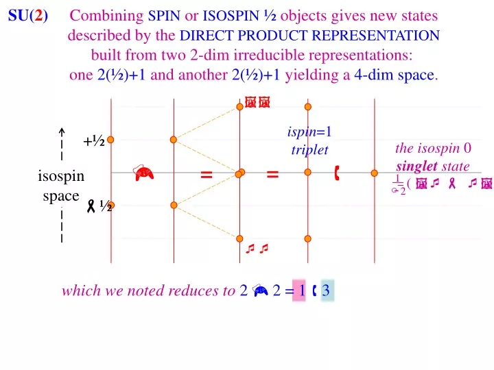
SU(2) Combining SPIN or ISOSPIN ½ objects gives new states described by the DIRECT PRODUCT REPRESENTATION built from two 2-dim irreducible representations: one 2(½)+1 and another 2(½)+1 yielding a 4-dim space. ispin=1 triplet +½ the isospin 0 singlet state = = isospin space 1 2 ( - ) -½ which we noted reduces to2 2 = 1 3
SU(2)- Spin added a new variable to the parameter space defining all state functions - it introduced a degeneracy to the states already identified; each eigenstate became associated with a 2+1multiplet of additional states - the new eigenvalues were integers, restricted to a range (- to + ) and separated in integral steps - only one of its 3 operators, J3, was diagonal, giving distinct eigenvalues. The remaining operators, J1 and J2, actually mixed states. - however, a pair of ladder operators could constructed: J+= J1 + iJ2 and J-= J1 - iJ2 which stepped between eigenstates of a given multiplet. n -1/2 +1/2 -1 0 1
The SU(3) Generators are Gi = ½i just like theGi = ½iare forSU(2) The ½ distinguishes UNITARY from ORTHOGONAL operators. iappear in the SU(2) subspaces in block diagonal form. 3’sdiagonal entries are just the eigenvalues of the isospin projection. 8is ALSO diagonal! It’s eigenvalues must represent a NEW QUANTUM number! Notice, like hypercharge (a linear combination of conserved quantities), 8 is a linear combinations of 2 diagonal matrices: 2 SU(2) subspaces.
The remaining matrices MIX states. In exactly the same way you found the complete multiplets representing angular momentum/spin, we can define T± G1± iG2 U± G6± iG7 V± G4± iG5 T±, T3are isospin operators By slightly redefining our variables we can associate the eigenvalues of 8 with HYPERCHARGE.
The COMMUTATION RELATIONS establish the stepping properties of these ladder (raising/lowering) operators T3|t3, y = t3|t3, y t3I3 Y|t3, y = y|t3, y Y U+ V+ T- T+ I3 U- V- =T+(T3+1)|t3, y T3(T+|t3, y) = (T+T3+T+)|t3, y = (t3+1)(T+|t3, y) Y(T+|t3, y) = T+(Y|t3, y) = y(T+|t3, y)
To be applicable to quantum mechanics, the lowest dimensional representation of SU(3) – the set of 3-dimensional matrices – must act on, and their eigenvalues describe, a set of real physical states,with quantum numbers: T3 = Y = ISO-SPIN I3+1/2 0 -1/2 HYPERCHARGE BARON NUMBER STRANGENESS CHARGE +1/3 -2/3 +1/3 +1/3 +1/3 +1/3 0 -1 0 +2/3 -1/3 -1/3 Q = I3 + ½Y Y B+S
Since Uis an assumed symmetry (mixing states within a multiplet but remaining invariant to strong interactions) consider: * e-iaG** which will also satisfy all the same equations as . Since Gi = -(Gi)* are obviously also traceless and hermitian (and satisfy the same algebraic Commutation Relations as theGi) we have a completely equivalent alternate set of generators for these SU(3) transformations ~ Mathematically we say we have a dual representation (or an adjunct basis set).
Physically we interpret this as another possible set of fundamental states carrying the minimum quanta of isospin and hypercharge, though now the eigenvalues (the diagonal elements of l3 and l8) change signs. Y +1 +1 down up s I3 -1 +1 -1 +1 u strange d -1 -1 The anti-particle quarks!
As m strictly adds when combining | j1m1 > | j2m2 > the quantum numbers t3 , ymust as well. Y +1 down up This quark multiplet simply plots the points representing the 3 possible quark states. I3 -1 +1 strange -1 A 2-quark state of up pairs would have a total t3=+1 and y=+2/3 Y Y +1 +1 up/up uu ud dn up d u I3 I3 -1 +1 -1 +1 us s s A ud state have a total t3=0 and y=+2/3 -1 -1
The 33=9 possible quark-quark states form 33= 36mulitplets Y +1 +1 +1 d u I3 -1 +1 -1 +1 -1 +1 s -1 -1 -1 Unfortunately the36mulitplets of quark-quark combinations include fractionally charged states, which do not seem to correspond to any known particles.
But by adding a 3rdquark (to the qq states we’ve built so far): +1 +1 -1 +1 -1 +1 -1 -1 Which we can directly compare to the knownspin-1/2baryons to these 63=18 qqq states which can be separated into 63= 810 mulitplets
the spin 3/2+ baryon decuplet the spin ½+ baryon octet n p - 0 + ++ +1 +1 - *- 0 + *0 *+ -1 +1 0 -1 +1 *- *0 -1 -1 - 0 -
Notice if you add a quark to an antiquark (or antiquark to a quark): +1 +1 -1 +1 -1 +1 -1 -1 33=9 new states are defined, separable into 33=18mulitplets to be compared directly to the known9spin-0and 9spin-1 mesons
the spin 1- meson nonet the spin 0- meson octet K0 K+ K*0 K*+ +1 +1 - - 0 + 0 + 0 0, 0 -1 +1 -1 +1 -1 -1 K- K0 K*- K*0
1974 Accelerators 1st breached the NEXT energy threshold and began creating NEW, HIGHER MASS particles! Endowed with another quantum number: CHARM requiring one more quark that carried it. As we will see later, by this time theorists had already extended u-d isospin symmetry into an anticipated s-c symmetry both subsets of larger SU(4) multiplets
c d u p0 p+ s p+ n p D- r0 D0 r- D+ D++ r+
Look at the FREE PARTICLE Dirac Lagrangian LDirac=iħcgm mc2 Dirac matrices Dirac spinors (Iso-vectors, hypercharge) Which is OBVIOUSLY invariant under the transformation ei (a simple phase change) because e-i and in all pairings this added phase cancels! This is just an SU(1) transformation, sometimes called a“GLOBAL GAUGE TRANSFORMATION.”
What if we GENERALIZEthis? Introduce more flexibility to the transformation? Extend to: but still enforce UNITARITY? eia(x) LOCAL GAUGE TRANSFORMATION Is the Lagrangian still invariant? LDirac=iħcgm mc2 (ei(x)) = i((x)) + ei(x)() So: L'Dirac = -ħc((x))gm +iħce-i(x)gm()e+i(x) mc2
L'Dirac = -ħc((x))gm+iħcgm() mc2 LDirac For convenience (and to make subsequent steps obvious) define: -ħc q (x) (x) then this is re-written as L'Dirac = +qgm()+LDirac recognize this???? the current of the charge carrying particle described by as it appears in our current-field interaction term
L'Dirac = +qgm()+LDirac If we are going to demand the complete Lagrangian be invariant under even such a LOCAL gauge transformation, it forces us to ADD to the “free” Dirac Lagrangian something that can ABSORB (account for) that extra term, i.e., we must assume the full Lagrangian HAS TO include a current-field interaction: L=[iħcgmmc2]-(qgm)Am defines its transformation and that under the same local gauge transformation
L=[iħcgmmc2]-(qgm)Am • We introduced the same interaction term 3 weeks back • following electrodynamic arguments (Jackson) • the form of the current density is correctly reproduced • the transformation rule • Am' = Am + l • is exactly (check your notes!) • the rule for GAUGE TRANSFORMATIONS • already introduced in e&m! The search for a “new”conserved quantum number shows that for an SU(1)-invariant Lagrangian, the freeDirac Lagrangain is “INCOMPLETE.” If we chose to allow gauge invariance, it forces to introduce a vector field (here that means Am) that “couples” to.
The FULL Lagrangian also needs a term describing the free particles of the GAUGE FIELD (the photon we demand the electron interact with). But wait! We’ve already introduced the Klein-Gordon equation for a massless particle, the result, the solution A = 0 was the photon field, A Of course NOW we want the Lagrangian term that recreates that! Furthermore we now demand that now be in a form that is both Lorentz and SU(3) invariant!
We will find it convenient to express this term in terms of the ANTI-SYMMETRIC electromagnetic field tensor More ELECTRODYNAMICS: The Electromagnetic Field Tensor but A=(V,A) and J=(c, vx, vy, vz) do! • E, B do not form 4-vectors • E, B are expressible in terms of and A the energy of em-fields is expressed in terms of E2, B2 • F = A-A transforms as a Lorentz tensor! = Ex since = Bz since
Actually the definition you first learned: In general = -Ex = -Bz Fik = -Fki= = 0 While vectors, like J transform as “tensors” simply transform as
x' = Lx or x = L-1x' Under Lorentz transformations
So, simply by the chain rule: and similarly:
(also xyzyzxzxy) both can be re-written with (with the same for xyz) All 4 statements can be summarized in
The remaining 2 Maxwell Equations: are summarized by ijk = xyz, xz0, z0x, 0xy Where here I have used the “covariant form” F= g g F=