Download
1 / 62
620 likes | 628 Views
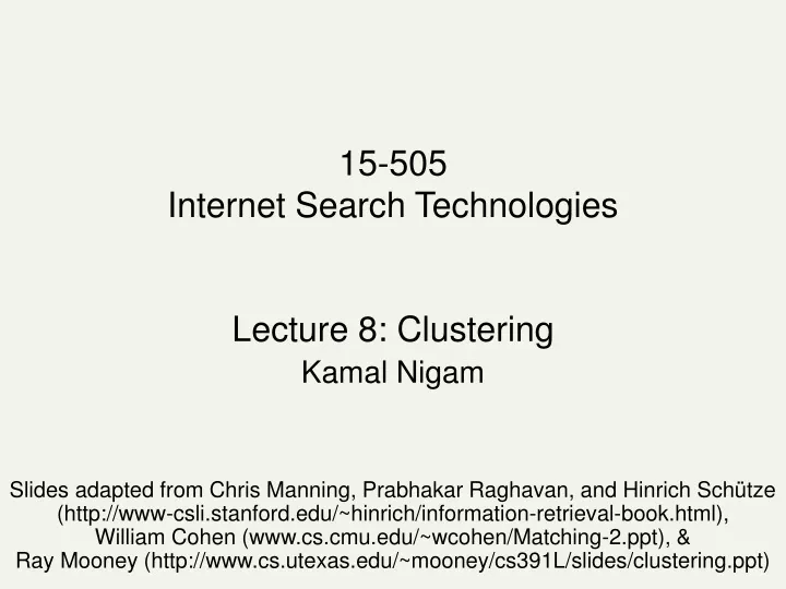
15-505 Internet Search Technologies. Lecture 8: Clustering Kamal Nigam

E N D
15-505Internet Search Technologies Lecture 8: Clustering Kamal Nigam Slides adapted from Chris Manning, Prabhakar Raghavan, and Hinrich Schütze (http://www-csli.stanford.edu/~hinrich/information-retrieval-book.html),William Cohen (www.cs.cmu.edu/~wcohen/Matching-2.ppt), & Ray Mooney (http://www.cs.utexas.edu/~mooney/cs391L/slides/clustering.ppt)
What is clustering? • Clustering: the process of grouping a set of objects into classes of similar objects • Most common form of unsupervised learning • Unsupervised learning = learning from raw data, as opposed to supervised data where a classification of examples is given
Clustering – Reference matching • Fahlman, Scott & Lebiere, Christian (1989). The cascade-correlation learning architecture. In Touretzky, D., editor, Advances in Neural Information Processing Systems (volume 2), (pp. 524-532), San Mateo, CA. Morgan Kaufmann. • Fahlman, S.E. and Lebiere, C., “The Cascade Correlation Learning Architecture,” NIPS, Vol. 2, pp. 524-532, Morgan Kaufmann, 1990. • Fahlman, S. E. (1991) The recurrent cascade-correlation learning architecture. In Lippman, R.P. Moody, J.E., and Touretzky, D.S., editors, NIPS 3, 190-205.
Clustering – Reference matching • Fahlman, Scott & Lebiere, Christian (1989). The cascade-correlation learning architecture. In Touretzky, D., editor, Advances in Neural Information Processing Systems (volume 2), (pp. 524-532), San Mateo, CA. Morgan Kaufmann. • Fahlman, S.E. and Lebiere, C., “The Cascade Correlation Learning Architecture,” NIPS, Vol. 2, pp. 524-532, Morgan Kaufmann, 1990. • Fahlman, S. E. (1991) The recurrent cascade-correlation learning architecture. In Lippman, R.P. Moody, J.E., and Touretzky, D.S., editors, NIPS 3, 190-205.
Clustering: Navigation of search results • For grouping search results thematically • clusty.com / Vivisimo
Clustering: Corpus browsing www.yahoo.com/Science … (30) agriculture biology physics CS space ... ... ... ... ... dairy botany cell AI courses crops craft magnetism HCI missions agronomy evolution forestry relativity
Clustering considerations • What does it mean for objects to be similar? • What algorithm and approach do we take? • Top-down: k-means • Bottom-up: hierarchical agglomerative clustering • Do we need a hierarchical arrangement of clusters? • How many clusters? • Can we label or name the clusters? • How do we make it efficient and scalable?
What makes docs “related”? • Ideal: semantic similarity. • Practical: statistical similarity • Treat documents as vectors • For many algorithms, easier to think in terms of a distance (rather than similarity) between docs. • Think of either cosine similarity or Euclidean distance
What are we optimizing? • Given: Final number of clusters • Optimize: • “Tightness” of clusters • {average/min/max/} distance of points to each other in the same cluster? • {average/min/max} distance of points to each clusters center? • Usually clustering finds heuristic approximations
Clustering Algorithms • Partitional algorithms • Usually start with a random (partial) partitioning • Refine it iteratively • K means clustering • Model based clustering • Hierarchical algorithms • Bottom-up, agglomerative • Top-down, divisive
Partitioning Algorithms • Partitioning method: Construct a partition of n documents into a set of K clusters • Given: a set of documents and the number K • Find: a partition of K clusters that optimizes the chosen partitioning criterion • Globally optimal: exhaustively enumerate all partitions • Effective heuristic methods: K-means algorithms
K-Means • Assumes documents are real-valued vectors. • Clusters based on centroids (aka the center of gravity or mean) of points in a cluster, c: • Reassignment of instances to clusters is based on distance to the current cluster centroids.
K-Means Algorithm Select K random seeds. Until clustering converges or other stopping criterion: For each doc di: Assign di to the cluster cjsuch that dist(xi, sj) is minimal. (Update the seeds to the centroid of each cluster) For each cluster cj sj = (cj) How?
Pick seeds Reassign clusters Compute centroids Reassign clusters x x Compute centroids x x x x K Means Example(K=2) Reassign clusters Converged!
Termination conditions • Several possibilities, e.g., • A fixed number of iterations. • Doc partition unchanged. • Centroid positions don’t change. Does this mean that the docs in a cluster are unchanged?
Convergence • Why should the K-means algorithm ever reach a fixed point? • A state in which clusters don’t change. • K-means is a special case of a general procedure known as the Expectation Maximization (EM) algorithm. • EM is known to converge. • Theoretically, number of iterations could be large. • Typically converges quickly
Time Complexity • Computing distance between doc and cluster is O(m) where m is the dimensionality of the vectors. • Reassigning clusters: O(Kn) distance computations, or O(Knm). • Computing centroids: Each doc gets added once to some centroid: O(nm). • Assume these two steps are each done once for I iterations: O(IKnm).
Seed Choice • Results can vary based on random seed selection. • Some seeds can result in poor convergence rate, or convergence to sub-optimal clusterings. • Select good seeds using a heuristic (e.g., doc least similar to any existing mean) • Try out multiple starting points • Initialize with the results of another method. Example showing sensitivity to seeds In the above, if you start with B and E as centroids you converge to {A,B,C} and {D,E,F} If you start with D and F you converge to {A,B,D,E} {C,F}
How Many Clusters? • Number of clusters K is given • Partition n docs into predetermined number of clusters • Finding the “right” number of clusters is part of the problem • Given data, partition into an “appropriate” number of subsets. • E.g., for query results - ideal value of K not known up front - though UI may impose limits. • Can usually take an algorithm for one flavor and convert to the other.
K not specified in advance • Say, the results of a query. • Solve an optimization problem: penalize having lots of clusters • application dependent, e.g., compressed summary of search results list. • Tradeoff between having more clusters (better focus within each cluster) and having too many clusters
K not specified in advance • Given a clustering, define the Benefit for a doc to be some inverse distance to its centroid • Define the Total Benefit to be the sum of the individual doc Benefits.
Penalize lots of clusters • For each cluster, we have a CostC. • Thus for a clustering with K clusters, the Total Cost is KC. • Define the Value of a clustering to be = Total Benefit - Total Cost. • Find the clustering of highest value, over all choices of K. • Total benefit increases with increasing K. But can stop when it doesn’t increase by “much”. The Cost term enforces this.
animal vertebrate invertebrate fish reptile amphib. mammal worm insect crustacean Hierarchical Clustering • Build a tree-based hierarchical taxonomy (dendrogram) from a set of documents. How could you do this with k-means?
Hierarchical Clustering algorithms • Agglomerative (bottom-up): • Start with each document being a single cluster. • Eventually all documents belong to the same cluster. • Divisive (top-down): • Start with all documents belong to the same cluster. • Eventually each node forms a cluster on its own. • Could be a recursive application of k-means like algorithms • Does not require the number of clusters k in advance • Needs a termination/readout condition
Hierarchical Agglomerative Clustering (HAC) • Assumes a similarity function for determining the similarity of two instances. • Starts with all instances in a separate cluster and then repeatedly joins the two clusters that are most similar until there is only one cluster. • The history of merging forms a binary tree or hierarchy.
Dendogram: Hierarchical Clustering • Clustering obtained by cutting the dendrogram at a desired level: each connected component forms a cluster.
Hierarchical Agglomerative Clustering (HAC) • Starts with each doc in a separate cluster • then repeatedly joins the closest pair of clusters, until there is only one cluster. • The history of merging forms a binary tree or hierarchy. How to measure distance of clusters??
Closest pair of clusters Many variants to defining closest pair of clusters • Single-link • Distance of the “closest” points (single-link) • Complete-link • Distance of the “furthest” points • Centroid • Distance of the centroids (centers of gravity) • (Average-link) • Average distance between pairs of elements
Single Link Agglomerative Clustering • Use maximum similarity of pairs: • Can result in “straggly” (long and thin) clusters due to chaining effect. • After merging ci and cj, the similarity of the resulting cluster to another cluster, ck, is:
Complete Link Agglomerative Clustering • Use minimum similarity of pairs: • Makes “tighter,” spherical clusters that are typically preferable. • After merging ci and cj, the similarity of the resulting cluster to another cluster, ck, is: Ci Cj Ck
Key notion: cluster representative • We want a notion of a representative point in a cluster • Representative should be some sort of “typical” or central point in the cluster, e.g., • point inducing smallest radii to docs in cluster • smallest squared distances, etc. • point that is the “average” of all docs in the cluster • Centroid or center of gravity
Centroid-based Similarity • Always maintain average of vectors in each cluster: • Compute similarity of clusters by: • For non-vector data, can’t always make a centroid
Computational Complexity • In the first iteration, all HAC methods need to compute similarity of all pairs of n individual instances which is O(mn2). • In each of the subsequent n2 merging iterations, compute the distance between the most recently created cluster and all other existing clusters. • Maintaining of heap of distances allows this to be O(mn2logn)
Major issue - labeling • After clustering algorithm finds clusters - how can they be useful to the end user? • Need pithy label for each cluster • In search results, say “Animal” or “Car” in the jaguar example. • In topic trees, need navigational cues. • Often done by hand, a posteriori. How would you do this?
How to Label Clusters • Show titles of typical documents • Titles are easy to scan • Authors create them for quick scanning! • But you can only show a few titles which may not fully represent cluster • Show words/phrases prominent in cluster • More likely to fully represent cluster • Use distinguishing words/phrases • Differential labeling • But harder to scan
Labeling • Common heuristics - list 5-10 most frequent terms in the centroid vector. • Drop stop-words; stem. • Differential labeling by frequent terms • Within a collection “Computers”, clusters all have the word computer as frequent term. • Discriminant analysis of centroids. • Perhaps better: distinctive noun phrase
Scaling up to large datasets • Fahlman, Scott & Lebiere, Christian (1989). The cascade-correlation learning architecture. In Touretzky, D., editor, Advances in Neural Information Processing Systems (volume 2), (pp. 524-532), San Mateo, CA. Morgan Kaufmann. • Fahlman, S.E. and Lebiere, C., “The Cascade Correlation Learning Architecture,” NIPS, Vol. 2, pp. 524-532, Morgan Kaufmann, 1990. • Fahlman, S. E. (1991) The recurrent cascade-correlation learning architecture. In Lippman, R.P. Moody, J.E., and Touretzky, D.S., editors, NIPS 3, 190-205.
Efficient large-scale clustering • 17M biomedical papers in Medline • Each paper contains ~20 citations • Clustering 340M citations • ~1017 distance calculations for naïve HAC
Expensive Distance Metric for Text • String edit distance • Compute with dynamic programming • Costs for character: • insertion • deletion • substitution • ...
String edit (Levenstein) distance • Distance is shortest sequence of edit commands that transform s to t. • Simplest set of operations: • Copy character from s over to t • Delete a character in s (cost 1) • Insert a character in t (cost 1) • Substitute one character for another (cost 1)
Levenstein distance - example • distance(“William Cohen”, “Willliam Cohon”) s alignment t op cost
Levenstein distance - example • distance(“William Cohen”, “Willliam Cohon”) s gap alignment t op cost
D(i-1,j-1), if si=tj //copy D(i-1,j-1)+1, if si!=tj //substitute D(i-1,j)+1 //insert D(i,j-1)+1 //delete = min Computing Levenstein distance D(i,j) = score of best alignment from s1..si to t1..tj
= D(s,t) Computing Levenstein distance