Download
1 / 18
180 likes | 254 Views
Solar Feature Catalogues. S Zharkov, V V Zharkova, S S Ipson, A.Benkhalil, N.Fuller, J. Aboudarham. EGSO SFC Specifications. Purpose Provide comprehensive information about: (a) features detected on a date; (b) provide a cropped image library;

E N D
Solar Feature Catalogues S Zharkov, V V Zharkova, S S Ipson, A.Benkhalil, N.Fuller, J. Aboudarham
EGSO SFC Specifications • Purpose • Provide comprehensive information about: (a) features detected on a date; (b) provide a cropped image library; • Create an option to search data by any feature characteristics • Feature automated detection (1996-2005) • Meudon daily Ca II K3 and H-alpha images (Plages and filaments) • SOHO/MDI white light images and magnetograms • Architecture • [ RDBMS ⇮ web services ⇮ web server ] under Linux • Data accessibility • EGSO broker: via web services [ASCII ⇮ to be extended to XML VOTable ] • Human user: via a web GUI [http://solar.inf.brad.ac.uk] • Special test features via web GUI • Preset searches for every feature by time, location, size, etc • Use cases for possible searches
Input Image Detected AR Chain Code Chain Code start pixel Chain Code constriction example Chain Code Directions • SSW software (EGSO branch): • Catalogue Search -> VOTable -> IDL SSW -> features reconstructed, over plotted
Catalogue Description (Zharkova et al., 2005, Sol.Phys.) • Observational Parameters: • Date of observation, resolution; determined quiet sun intensity; • Feature Parameters: • Gravity center (proj & Carrington), area, diameter, umbra size, bounding rectangle, intensity statistics, magnetic information • Filaments: skeleton center, elongation, curvature • Raster Scans (bounding rectangle mask): • reconstructed: pixel values equal to 0 corresponding to quiet Sun, 1 to penumbra, 2 to umbra • Chain Codes: filaments, filament skeletons, plages • Sunspot Catalogue (from 1996-05-19 19:08:35 to 2005-05-31 19:51:32) • About 10000 observation processed • ~370000 sunspots and 100 000 ARs stored • SSW software: • Catalogue Search -> VOTable -> IDL SSW -> features reconstructed, over plotted
Techniques for filament recognition • Training the ANNs: • Different conditions (brightness, variable background, inhomogeneity in the solar atmosphere etc) • Representative training dataset (not so many examples are available, solar images are still labelled manually) • Morphological operations: • a quick look technique • Thresholding and region growing • ANNs ANN: V.V.Zharkova, V.Schetinin, Sol.Phys. (2005)228 RegionGrowing:Fuller, Aboudarham, Bentley:Solar Phys. (2005)227
ANN Method V.V.Zharkova, V.Schetinin, Sol.Phys. (2005)228 • The output of the first hidden neuron sj = f1(w0(1), w(1); z(j)), j = 1…q, (1) • where w0(1) is a bias, w(1) is a weight vector and f1 is the activation function of the neuron. • The output of the second hidden neuron is proportional to the brightness of a background: uj = f2(w0(2), w(2); j), j = 1…q, (2) • here the w0(2) and w(2) are defined so that the output u is the evaluation of a background component contributed to the pixels of the column z(j). These parameters learnt from the image data. • Taking the outputs sj and uj, the output neuron makes a decision yj (0, 1) for column vector z(j): yj = f3(w0(3), w(3); sj, uj), j = 1…q. (3)
A Parabolic Approximation The recognized filament (in black) An original filament fragment The parabolic approximation of output uj, Output sj Normalised uj - sj
Filament detectionFuller, Aboudarham, Bentley:Solar Phys. (2005)227 * 89 % of the 'automatic' filaments match the 'manual' ones. * 4 % of the 'automatic' filaments don't correspond to 'manual' ones. In fact, most of them have not been manually detected, but a careful inspection shows that they are real filaments but faint ones most of the time. * 11 % of 'manual' filaments haven't been automatically detected. But the error in the total length of all filaments is only 7 % (i.e. non detected filaments were small ones). Again, when carefully looking at these filaments, it appears that these are also faint ones in general.
The pruned skeleton • The thinning morphological operator is used to get the skeleton of the binary blob (1). The result is the skeleton of the object (2 with dashed line for the boundary). It contains many short branches produced by small irregularities on the boundary of the object. An algorithm, calculating the distances between nodes and branches pixels, has been developed to remove the branches, keeping the full length skeleton (3). The following descriptive parameters can be deduced from the skeleton: • - The length • - The filament centre as the middle of the skeleton, in heliographic coordinates or in pixels • - A curvature index • The chain code of the skeleton can also be computed to get a linear representation of the filament.
Magnetic inversion line and filament skeleton comparison Comparison of solar filament elongations extracted from SFC and LOS magnetic inversion lines, 551 filaments from 14 Halpha images Ipson et al, Solar Phys. (2005)228 MNL detection: 2D gaussian smoothing, examine each pixel for change of sign (8neighbours) thinning procedure followed by segmentation into connected objects
Inversion line detection Three main stages Voronoi Tessellation and Line map Median Filter and Threshold Output Neutral line Map Euclidian Distance Transform Input magnetogram
Inversion line detection Median filter and threshold at 20 G Distance Transform Boundaries between positive and negative regions marked Pixels labelled according to nearest magnetic polarity
Sunspot Detection:Zharkov et al, SolarPhys (2005):228 detected edges & low int regions => <= original image <ROI result >
http://solar.inf.brad.ac.uk Thank You!