Download
1 / 21
220 likes | 467 Views
From Lotka-Volterra to mechanism: . Simple models have advantages: capturing essential features of dynamical systems with minimal mathematical effort tractable, relatively easy to analyze in full can be parameterized from observation However, they have limited utility:

E N D
From Lotka-Volterra to mechanism: • Simple models have advantages: • capturing essential features of dynamical systems with minimal mathematical effort • tractable, relatively easy to analyze in full • can be parameterized from observation • However, they have limited utility: • Parameter values are difficult to predict a prior from knowledge of the system
Example: r1 = 0.12 K1 = 170 a = 0.9 r2 = 0.09 K2 = 170 b = 0.5
Hierarchy of explanation Changes in population size (population dynamics) births deaths migrations Energy balance: food availability maintenance cost cost of reproduction Risk factors: predator encounters disease exposure physical conditions Behavior: dispersal foraging group dynamics
Empirical models: The observations required to estimate parameters are the very same that the model predicts (parameterization = calibrating, fitting). observation Population changes through time MODEL prediction parameter estimation
Mechanistic models: Some of the observations required to estimate parameters are at least one step removed from the level of prediction. observation Population changes through time MODEL parameter estimation prediction
Tilman’s resource ratio model of plant competition Observations used to parameterize the model describe resource uptake by plants. Hence, this is a mechanistic model. is the minimal amount Of resource species A requires to persist in an environment; If RA is supplied at a certain rate, the species should increase until the resource concentration reaches exactly this value. loss Species A growth Biomass growth or loss rate loss Resource level
Tilman’s resource ratio model of plant competition loss loss Species A Species B growth Biomass growth or loss rate loss When two species are competing for a single limiting resource, the species with the lower equilibrial resource requirement should completely replace the other (B outcompetes A) Resource level Resource level
Species could be competing for two resources: loss loss Species A Species A growth Biomass growth or loss rate loss Resource 1 level at fixed value of Resource 2 Resource 2 level at fixed value of Resource 1
Species depend on different resources in different ways: The zero-net-growth-isoclines (ZNG’s) R2 R2 R2 R2* R1 R1 R1 R1* Resources are perfectly essential Resources are complementary Resources are perfectly substitutable
Adding resource dynamics R2 Resource consumption vector Resource supply point; what resources would be without uptake Resource supply vector R1
At equilibrium, both consumers and resources must be unchanging. Thus, resource supply = resource demand: R2 This is where consumer and resource are at equilibrium Resource consumption vector Resource supply point; what resources would be without uptake Resource supply vector R1
Prediction: if different habitats have different resource supply points, resource levels at equilibrium will be different. R2 Resource consumption vector Resource supply point; what resources would be without uptake Resource supply vector R1
Species with different resource requirements affect resource levels differently: R2 R1 R1
What if two species with different resource requirements inhabit the same habitat? R2 R1 R1
What if two species with different resource requirements inhabit the same habitat? R2 R1 R1
A two-species equilibrium must be located on both species’ ZNG’s A and B coexist R2 B A R1 R1
Habitat determines if coexistence is possible. B wins, because it can draw R1 to levels intolerable to A. R2 B A R1 R1
Habitat determines if coexistence is possible. A wins, because it can draw R2 to levels intolerable to B. R2 B A R1 R1
Habitat determines if coexistence is possible. A wins, because it can draw R2 to levels intolerable to B. R2 Species A & B coexist Species B wins Species A wins B A Both species die R1 R1
Tilman’s model still predicts the four outcomes of competition that the Lotka-Volterra model does, and one more: no species lives A always wins B always wins A B B A A & B can coexist in some habitats A & B can coexist in some habitats B always wins A always wins B B A A
Summary: What do we gain from Tilman’s more mechanistic model? • Resource requirements for growth can be tested independently of competition. • New predictions: the effect of habitat on species interaction. • Previously overlooked outcomes: both species can fail. • There are predictions we can test and which can fail. • Because the model is process based, we can more easily expand the model to add more realism.