Download
1 / 49
490 likes | 585 Views
Stochastic Control of Heterogeneous Networks. Eytan Modiano Massachusetts Institute of Technology. http://web.mit.edu/modiano/www. Outline. Introduction Optimal power and rate allocation Joint routing and power allocation Joint flow control, routing and power allocation

E N D
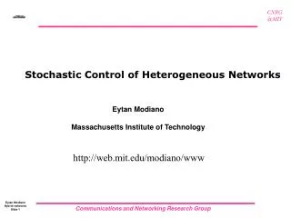
Stochastic Control of Heterogeneous Networks Eytan Modiano Massachusetts Institute of Technology http://web.mit.edu/modiano/www
Outline • Introduction • Optimal power and rate allocation • Joint routing and power allocation • Joint flow control, routing and power allocation • Distributed Implementations • Summary
Hybrid space-terrestrial networks • Networks must be designed to work effectively across heterogeneous component • Architecture must be scalable, robust and cost effective (from access to backbone) • Resource utilization must be very efficient (especially for space and wireless segments)
Research Overview • High-speed optical networks (NSF, DARPA, DTRA) • WDM network architecture • Optical bypass of the electronic layer • Network survivability • Satellite networks (NASA, DARPA, NRO) • Resource allocation in next generation satellite networks • Hybrid space-terrestrial networking • LEO satellite networks • Wireless ad-hoc networks (Draper labs, Samsung, DARPA, AFOSR, ONR, NSF) • Autonomous networks of air and ground vehicles • Distributed sensor networks
Outline • Introduction Optimal power and rate allocation • Joint routing and power allocation • Joint flow control, routing and power allocation • Distributed Implementations • Summary
SATELLITE R1(t) 1 1 VIRTUAL OUTPUT BUFFERS XMTR N RN(t) N TIME-VARYING CHANNEL Scheduling with multiple downlink beams • Satellite to ground channel or wireless (cellular) downlink • Time varying channel quality • Random traffic arrivals • Allowable transmission rates limited by • Number of transmitters • Total available power • Bandwidth DOWNLINK BEAMS Throughput optimal scheduling • Want to keep the system stable => bounded average queue occupancy • Stabilizing algorithm => maintains stability whenever possible • Single transmitter & non-time-varying channels • Serving the fastest queue (channel) minimizes buffer occupancy => maintains stability • What happens with multiple transmitters? • What if the channels are time-varying?
l = p packets/slot l = p packets/slot R = 2 packets/slot R = 2 packets/slot 1- p2 + e packets/slot R = 1 packet/slot Instability of fastest queue first(non time varying channel) Two servers, Bernoulli arrivals • When packets arrive to either of the top two queues they are served first • With probability p2 no server can serve last queue • As long as arrival rate exceeds 1 - p2 last queue is unstable • Notice that when p < 1, if we assign one server to always serve queue 3 and the other to alternate between 1 and 2, all queues would be stable
R(p,c3) R(p,c2) Ri R(p,c1) Pi improving channel conditions Optimal Power Allocation(time varying channel) • Ri(Pi(t), Ci(t)) - Rate for user i when channel state is Ci and Pi power allocated • Theorem 1: Throughput optimal algorithm allocates power during time-slot t according to: • Generalization of TE92 max-weight rule to power allocation Limit on total allocated power : Arrival and channelstatistics are not known Ui - buffer occupancy; Pi - allocated power; Ci - channel state Michael Neely, Eytan Modiano and Charles Rohrs, "Power Allocation and Routing in Multi-BeamSatellites with Time Varying Channels," IEEE Transactions on Networking, February, 2003
Generalization to optimal rate (or bandwidth) allocation • In many situations power cannot be split across beams • Equivalent problem of allocating rate between the beams through time or frequency sharing • Throughput optimal rate allocation:“Max weight rule” • Similar result applies to general rate allocation regions • Application to future military satellite system - Lincoln Laboratory • Complex allocation of time slots, frequencies, modes, etc. A. Narula-Tam , T. G. Macdonald , E. Modiano , L Servi, “A Dynamic Resource Allocation Strategy for Satellite Communications,” IEEE MILCOM, October, 2004.
Proof of stability • Proof: Using Lyapunov stability
Numerical Example • Time-varying channel model • 3 States: Log-Normal attenuation • Good: SNR = 15 dB • Medium: SNR = 10 dB • Bad: SNR = 0 dB • Transition between states according to a Markov chain • Rate power curves using the Shannon capacity formula
Outline • Introduction • Optimal power (or rate) allocation Joint routing and power allocation • Joint flow control, routing and power allocation • Distributed Implementations • Summary
Route 1 Packets Route 2 Route 3 Joint routing and power allocation • Multiple routes to destination • Stabilizing routing and power allocation • Route packets to shortest queue (regardless of channel state) • Allocate power according to power allocation of Theorem 1 • Can be generalized to arbitrary activation sets • Each packets can be routed to a subset of the queues • Power is shared among different subsets of queues • Not all queues can be activated simultaneously
Extension to wireless networks • Transmission rates along the different links is a function of the power allocated to the links • Can model interference and mobility • Given a traffic demand (perhaps unknown) between nodes in the network, how do we route packets and allocate power to maximize the network capacity? Time varying channel
c c a b Optimal routing and power allocation • Each commodity C {1,..,N} corresponds to data associated with a given destination node • Routing algorithm - along each link (a,b) route commodity C that maximizes the differential backlog along that link [TE92]. i.e., • Algorithms uses “back pressure” to find the routes • Power allocation: • Generalization of [TE92] max-weight activation set algorithm to power allocation • Only a subset of the links can be activated simultaneously Michael Neely and Eytan Modiano, “Dynamic Power Allocation and Routing for Time Varying Wireless Networks ,” IEEE Journal on Selected Areas in Communications, January, 2005.
W = max(3,1) = 3 3 3 1 1 1 1 2 1 0 2 2 1 2 3 2 3 2 Differential Backlog Routing • Example – primary interference 7 6 6 6 6 1 6 4 7 3 2 6 7 7 6 7 8 6 7 7 7 6
Example: Mobile ad hoc network 10 nodes, 5x5 grid Users move between cells according to a Markov mobility model Power attenuation loss as d4 CDMA interference model: - Rate function of SINR Comparison to 2-hop relay algorithm (Grossglauser-Tse)
Outline • Introduction • Optimal power (or rate) allocation • Routing and power allocation Joint flow control, routing and power allocation • Distributed Implementations • Summary
Flow Control • When demand exceeds the system capacity • Queues build up • data discarded • congestion increases => instability • Flow control is needed to regulate traffic flow • Flow control prevents network instability by keeping packets waiting outside the network rather than in queues inside the network • Objectives of flow control • Maximize network throughput • Reduce network delays • Maintain quality-of-service parameters • Fairness, delay, etc.. • Tradeoff between fairness, delay, throughput… Which packets should be dropped? Or not admitted?
Optimal flow control • Let ri be the data rate allocated to session i (steady state), • Let gi(r) be the “utility” of allocating rate r to session i • Optimal flow control objective: maximize sum utilities subject to capacity constraints • Can be used to model a wide range of QoS objectives • In principle, if the arrival rates, channel statistics and network capacity region were all known above optimization can be solved • In practice we don’t usually know the network capacity region • Even the arrival rates and channel statistics are often unknown • Need a dynamic control strategy
l2 0.6 Pr[ON] = p1 l1 l2 l1 Pr[ON] = p2 0.5 Example: one server, 2 queue downlink, ON/OFF channels P1 = 0.5 P2 = 0.6 Capacity region L: • Throughput optimal algorithm (serve ON queue with largest backlog) • Stabilizes whenever rates are strictly interior to L • What happens when rates are outside L ?
Comparison of dynamic control algorithms Throughput optimal max-weight rule (max Uimi) Borst Alg. [Borst Infocom 2003] (max mi/mi) Tse Alg. [Tse 97, 99, Kush 2002] (max mi/ri)
Flow regulator Overflow buffer Network buffers Flow control mechanism • Put data into reservoir (overflow buffer) • Valve controls how much data to admit during each time-slot (Ric(t)) • Once data inside the network - use the same routing and rate allocation schemes as before • Max weight rate allocation • Max differential backlog routing • Optimal choice of Ric(t) values achieves maximum utility values Michael Neely, Eytan Modiano and C. Li, “Fairness and optimal stochastic control of heterogeneous networks,”IEEE/ACM Transactions on Networking, to appear.
Dynamic control strategy • Optimal Flow control: pick Ric(t) • Threshold rule that depends on the amount of data in the buffer (U) • The amount of data allowed into the network depends on the buffer levels • V is a control parameter that affects the performance of the algorithm • Large V => More delay but higher throughput • Algorithm comes arbitrarily close to the optimal operating point • Proof uses Lyapunov stability theory • Algorithm is a dynamic, decentralized control algorithm that does not require knowledge of the traffic and channel statistics • Trivial implementation - does not require solution to a complex optimization • Each node makes independent decisions Max : Subject to : for all c Michael Neely, Eytan Modiano and C. Li, “Fairness and optimal stochastic control of heterogeneous networks,”IEEE/ACM Transactions on Networking, to appear.
Examples of rule • Maximum throughput and the threshold rule • Proportional fairness and the 1/U rule Linear utilities: gnc(r) = anc r Logarithmic utilities: gnc(r) = log(1 + rnc)
optimal point r* Performance of algorithm l1 • V is a control parameter that affects the performance of the algorithm • Large V => More delay but higher throughput • Algorithm comes arbitrarily close to the optimal operating point Utility (throughput): Buffer occupancy (Delay): C1, C2 constants
Simulation Results(ON/OFF downlink example from before) a)g1(r)=g2(r)= log(1+r) b)g1(r)=log(1+r) g2(r)=1.28log(1+r) (priority service) l1= 0.5 packets/slot, l2 = 1 packet/slot; r* = (0.23, 0.57)
Performance: example(two users, on-off channel) User 1: ON with probability 0.5; User 2: ON with probability 0.6 g1(r)= log(1+r); g2(r)= 1.3log(1+r) l1= 0.5 packets/slot, l2 = 1 packet/slot; r* = (0.23, 0.57) Data rates Buffer occupancy (delay)
Outline • Introduction • Optimal power (or rate) allocation • Routing and power allocation • Joint flow control, routing and power allocation Distributed Implementations • Summary
Throughput Maximization in Wireless Networks • Routing: Maximum Differential Backlog [TE92] • Scheduling: Only a subset of the links can be activated simultaneously • Maximum Weight Activation Set • Weights are the backlogs 2 • Single hop traffic - scheduling • Find a Maximum Weight activation setin every time slot • Weights – Queue sizes • Primary interference constraints • A node transmits to a single neighbor at a time • Multiple transmissions can take place as long as they do not share a common node • Find a Maximum Weight Matching (O(n3)) in every time slot 4 3 NP-Complete 1 6 Centralized 5 7 8 High complexity
Distributed Solutions • In wireless networks there is a need for distributed solutions • Unlike in switches/routers • The optimization problem cannot be solved in a distributed manner every slot/frame • Recent distributed scheduling schemes • Lin and Shroff (2005) Chaporkar et al. (2005, 2006), Wu and Srikant (2005), Chen et al. (2006) • Maximal weight (greedy) matching or Maximal matching • Instead of Maximum Weight Matching • Guarantee only 50% throughput 2 4 3 1 6 5 7 8
Randomized Algorithms • In a centralized setting randomized algorithms can obtain 100% throughput (Tassiulas, 1998) • Algorithm • S(t)is the schedule (matching) at timet • At timet + 1 choose a matchingR(t +1)randomly from all possible matchings • S(t +1)is the heaviest betweenS(t)andR(t +1) • Conditions on the random selection S(t) R(t+1) Max {S(t) , R(t +1)} Centralized R(t+1) S(t+1) S(t) Weight Matchings
Framework for distributed scheduling in a wireless network NEW-SCH • Distributed Framework • S(t)is the schedule (matching) at timet • At timet +1 randomly obtain a matchingR(t+1)by a distributed algorithm NEW-SCH • S(t +1)is obtained by a distributed algorithm MIXusing inputsS(t)andR(t+1) MAX MIX • MIX • Combines both matchings • S(t +1) is not necessarily the heaviest matching S(t) R(t +1) MIX{S(t) , R(t +1)} 2 4 3 1 6 5 7 8
Ideal Weight With low probability S(t) R(t+1) Max Matchings MIX MIX MIX MIX 2 4 • Combines both matchings • Combined weight may be below maximum • Provides framework for distributed algorithms • Allows for decentralized operation in different parts of the network • No need for exact maximum and global knowledge • “Errors” are allowed - enables inaccurate computation 3 1 6 5 7 8
Stability Region • Theorem: Let NEW-SCH and MIX satisfy: • The probability that NEW-SCH selects the Maximum Weight Matching is d> 0 • The probability that following MIX Weight of S(t +1) (1- g) Max {Weight of S(t), Weight of R(t +1)} is 1-d1(d1<<d) Then, the network is stable for any set of rates • The constants d , d1 , g • Affect the stability region • Affect the complexities (L*- the stability region under centralized scheduler) Tradeoffs Design of algorithms
Obtaining a New Schedule (NEW-SCH) • A Maximal Matching algorithm that has a positive probability (d) to find the Maximum Weight Matching • Israeli and Itai, 1986 • A constant number of iterations is required to guarantee that d > 0 • Mix depends on the interference models • Focus: primary interference constraints • General interference and multi-hop traffic E. Modiano, D. Shah, and G. Zussman, “Maximizing Throughput in Wireless Networks via Gossiping,” Proc. ACM SIGMETRICS / IFIP Performance'06, June 2006. (Winner of Best Paper Award) A. Eryilmaz, E. Modiano, and A. Ozdaglar, “Distributed Control for Throughput-Optimality and Fairness in Wireless Networks,” Proc. of CDC, December 2006. A. Eryilmaz, A. Ozdaglar, E. Modiano, "Polynomial Complexity Algorithms for Full Utilization of Multi-hop Wireless Networks", IEEE Infocom, May 2007.
Combining the Schedules (MIX) • The combination of the current (S(t)) and random (R(t +1)) matchings creates connected components • An independent decision has to be made in each component (MIX) • Not necessarily simultaneously • Within a component • Nodes need to collect the sums of weights • Need to make the same decision • No node needs global information Paths Cycles C S ( t ) 1 R ( t + 1 ) C 2
Distributed MIX Algorithm - Deterministic • Mixing is simple on a path – the end nodes can become “leaders” • On a cycle • Every node sends a summation packet that collects the sums of weights along the cycle • The packet halts at the initiating node • Each node makes a decision based on “its” packet • If Weight [R(t+1)] > Weight [S(t)]Change to R(t+1) • Otherwise, stay with S(t) • Requires node identities to determinethat packet has returned to its source 2 4 3 1 6 5 7 8
Distributed MIX Algorithm - Deterministic • Recall that if following MIX the probability that Weight of S(t +1) (1- g) Max {Weight of S(t), Weight of R(t +1)} is 1-d1 Then, the network is stable for any set of rates (L* - the stability region under perfect/centralized scheduler) • With the deterministic MIX, the decision is exact • g = 0, d1 = 0 • Time complexity - O(L) • Communication complexity - O(L2) L – path length (in the worst case – the number of nodes)
2 4 Distributed MIX - RandomizedGossip Algorithms • Gossip algorithms disseminate information in a randomized manner • Karp et al. (2000), Kempe et al. (2003),Boyd et al. (2005), Ganesh et al. (2005) • Compute functions of network variables • E.g., averages • Tradeoff between running time and accuracy • Used in each component (cycle) • Estimate the weights of the current (S(t)) and random (R(t+1)) matchings 1 3 5
Simple Gossip Mechanism • Within a cycle • Estimates the weights of S(t) and R(t+1) • Xv(0) – node v’s weight at time 0 • Xv(i) – node v’s estimate of the average weight at iteration i • Each node contacts a neighbor with probability ½ • If decides to contact, selects one of the neighbors randomly • If u is contacted by v • If u decided to contact v, they average their values:Xu(i) = Xv(i) = AVG [Xv (i – 1) , Xv (i – 1)] • Stop after I(L) = Q(L2[ – log d2 – log e])iterations
Gossip Mechanism I (cont.) • Lemma: At the end of iteration I(L) • The estimates will be close to the exact value • The estimates at different nodes of may differ Some nodes may prefer the new matching while others retain the current one Need a mechanism that will ensure a synchronized decision (agreement) • If a node in the cycle decides differently than its neighbor • The current schedule (S(t)) is retained • If there are no differences • Follow the decision
Gossip and Agreement • Lemma: If Pr(All nodes move toR(t +1)) 1 – 2d2 • Recall (theorem) that if the probability that following MIX Weight of S(t +1) (1- g) Max {Weight of S(t), Weight of R(t +1)} is 1-d1(d1<<d) Then, the network is stable for • The choice of d2 and eaffect the complexity of the algorithm • Selection of d2 and e leads to a stability region (1 –a – b )L* • a and b - small constants • Affect the number of iterations • Do not affect the complexities • We use the fact that some inaccuracy is allowed
Comparison of various algorithms n – number of nodes, |E| - number of edges, a, b – small constants
3 4 Extensions - General Interference Constraints • Primary interference constraints are not realistic in many settings • Under general interference constraints a link can be active if other links are not active • Not necessarily adjacent • May depend on geographical structure, SNR, etc. • An interference/conflict graph can be derived from the network graph • Neighboring nodes represent interfering links 2,3 3,5 1,2 5 1 2 2,4 4,5
General Interference Constraints (Cont.) • For maximum throughput [TE92] • In every slot - find Maximum Weight Independent Set in the interference graph • NP-Complete • Not amendable to distributed implementation • The randomized framework still works • Randomly find a Maximal independent set • Mix current and random schedules • Although the basic scheduling problem is NP-Complete, randomized algorithms enable to obtain maximum throughput distributedly A. Eryilmaz, A. Ozdaglar, E. Modiano, "Polynomial Complexity Algorithms for Full Utilization of Multi-hop Wireless Networks", IEEE Infocom, May 2007.
Summary • Cross-layer resource allocation critical for making efficient use of network resources • Developed stochastic control framework that provides Joint scheduling, routing and flow control in a heterogeneous network • Novel flow control scheme that maximizes network utility • Developed a distributed framework for resource allocation in wireless networks • Based on randomized algorithms • “graph models” for wireless networks • E.g., primary interference • Future work • Extension to general interference models • Deterministic schemes: • E.g., A partitioning approach (Brzezinski, Zussman, and Modiano - ACM Mobicom’06) • In which graphs maximal-scheduling can achieve 100% throughput ? • How to partition the network into such sub-graphs ?