Economics 105: Statistics

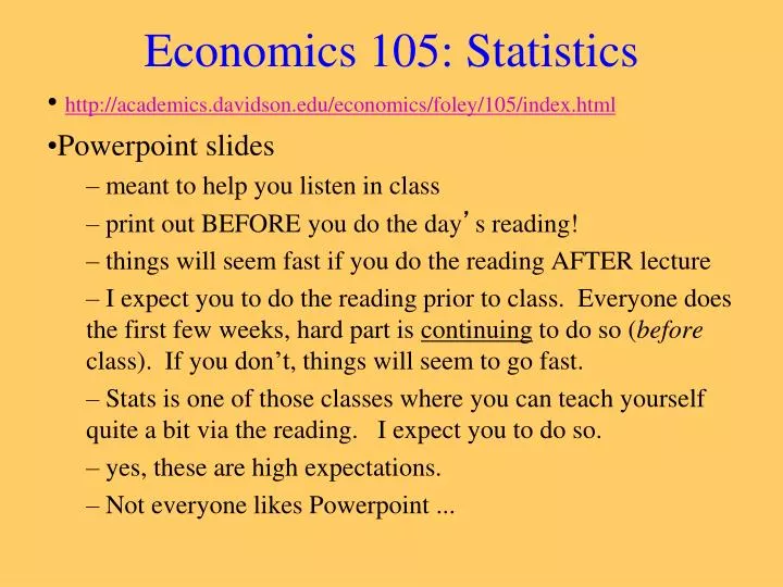
1. Economics 105: Statistics http://academics.davidson.edu/economics/foley/105/index.html Powerpoint slides meant to help you listen in class print out BEFORE you do the day’s reading! things will seem fast if you do the reading AFTER lecture I expect you to do the reading prior to class. Everyone does the first few weeks, hard part is continuing to do so (before class). If you don’t, things will seem to go fast. Stats is one of those classes where you can teach yourself quite a bit via the reading. I expect you to do so. yes, these are high expectations. Not everyone likes Powerpoint ...

2. Economics 105: Statistics Today What is Statistics? Presenting data For next time: Read Chapters 1 – 3.5

3. Organizing and Presenting Data Graphically Data in raw form are usually not easy to use for decision making Some type oforganizationis needed Table Graph Techniques reviewed in Chapter 2: Bar charts and pie charts Pareto diagram Ordered array Stem-and-leaf display Frequency distributions, histograms and polygons Cumulative distributions and ogives Contingency tables Scatter diagrams

4. Raw Form of Data Example: A manufacturer of insulation randomly selects 20 winter days and records the daily high temperature 24, 35, 17, 21, 24, 37, 26, 46, 58, 30, 32, 13, 12, 38, 41, 43, 44, 27, 53, 27

5. Tabulating Numerical Data: Frequency Distributions What is a Frequency Distribution? A frequency distribution is a list or a table … containing class groupings (ranges within which the data fall) ... and the corresponding frequencies with which data fall within each grouping or category Why use one? Useful, quick, visual summary of the data

6. Class Intervals and Class Boundaries • Each class grouping has the same width • Determine the width of each interval by • Usually at least 5 but no more than 15 • Class boundaries never overlap • Round up the interval width to get desirable endpoints

7. Frequency Distribution Example (continued) • Sort raw data in ascending order:12, 13, 17, 21, 24, 24, 26, 27, 27, 30, 32, 35, 37, 38, 41, 43, 44, 46, 53, 58 • Find range: 58 - 12 = 46 • Select number of classes: 5(usually between 5 and 15) • Compute class interval (width): 10 (46/5 then round up) • Determine class boundaries (limits): • 10, 20, 30, 40, 50, 60 • Compute class midpoints: 15, 25, 35, 45, 55 • Count observations & assign to classes

8. Frequency Distribution Example (continued) Data in ordered array: 12, 13, 17, 21, 24, 24, 26, 27, 27, 30, 32, 35, 37, 38, 41, 43, 44, 46, 53, 58 Relative Frequency Class Frequency Percentage 10 but less than 20 3 .15 15 20 but less than 30 6 .30 30 30 but less than 40 5 .25 25 40 but less than 50 4 .20 20 50 but less than 60 2 .10 10 Total 20 1.00 100

9. Tabulating Numerical Data: Cumulative Frequency Data in ordered array: 12, 13, 17, 21, 24, 24, 26, 27, 27, 30, 32, 35, 37, 38, 41, 43, 44, 46, 53, 58 Cumulative Frequency Cumulative Percentage Class Frequency Percentage 10 but less than 20 3 15 3 15 20 but less than 30 6 30 9 45 30 but less than 40 5 25 14 70 40 but less than 50 4 20 18 90 50 but less than 60 2 10 20 100 Total 20 100

10. Graphing Numerical Data: The Histogram • A graph of the data in a frequency distribution is called a histogram • The class boundaries(orclass midpoints) are shown on the horizontal axis • the vertical axisis eitherfrequency, relativefrequency,orpercentage • Bars of the appropriate heights are used to represent the number of observations within each class

11. Histogram Class Midpoint Class Frequency 10 but less than 20 15 3 20 but less than 30 25 6 30 but less than 40 35 5 40 but less than 50 45 4 50 but less than 60 55 2 (No gaps between bars) Class Midpoints

12. Graphing Numerical Data: The Frequency Polygon Class Midpoint Class Frequency 10 but less than 20 15 3 20 but less than 30 25 6 30 but less than 40 35 5 40 but less than 50 45 4 50 but less than 60 55 2 (In a percentage polygon the vertical axis would be defined to show the percentage of observations per class) Class Midpoints

13. Graphing Cumulative Frequencies: The Ogive (Cumulative % Polygon) Lower class boundary Cumulative Percentage Class Less than 10 0 0 10 but less than 20 10 15 20 but less than 30 20 45 30 but less than 40 30 70 40 but less than 50 40 90 50 but less than 60 50 100 Class Boundaries (Not Midpoints)

14. Summary Measures Describing Data Numerically Central Tendency Quartiles Variation Shape Arithmetic Mean Range Skewness Median Interquartile Range Mode Variance Geometric Mean Standard Deviation Coefficient of Variation

15. Measures of Central Tendency Overview Central Tendency Mode Geometric Mean Arithmetic Mean Median Midpoint of ranked values Most frequently observed value

16. Arithmetic Mean • The arithmetic mean (mean) is the most common measure of central tendency • For a sample of size n: Sample size Observed values

17. Arithmetic Mean (continued) • Mean = sum of values divided by the number of values • Affected by extreme values (outliers) 0 1 2 3 4 5 6 7 8 9 10 0 1 2 3 4 5 6 7 8 9 10 Mean = 3 Mean = 4

18. Median • In an ordered array, the median is the “middle” number (50% above, 50% below) • Not affected by extreme values 0 1 2 3 4 5 6 7 8 9 10 0 1 2 3 4 5 6 7 8 9 10 Median = 3 Median = 3

19. Finding the Median • The location of the median: • If the number of values is odd, the median is the middle number • If the number of values is even, the median is the average of the two middle numbers • Note that is not the value of the median, only the position of the median in the ranked data

20. Mode • A measure of central tendency • Value that occurs most often • Not affected by extreme values • Used for either numerical or categorical (nominal) data • There may may be no mode • There may be several modes 0 1 2 3 4 5 6 0 1 2 3 4 5 6 7 8 9 10 11 12 13 14 No Mode Mode = 9

21. Five houses on a hill by the beach Review Example House Prices: $2,000,000 500,000 300,000 100,000 100,000

22. Mean: ($3,000,000/5) = $600,000 Median: middle value of ranked data = $300,000 Mode: most frequent value = $100,000 Review Example:Summary Statistics House Prices: $2,000,000 500,000 300,000 100,000 100,000 Sum $3,000,000

23. Meanis generally used, unless extreme values (outliers) exist Then medianis often used, since the median is not sensitive to extreme values. Example: Median home prices may be reported for a region – less sensitive to outliers Which measure of location is the “best”?

24. Geometric Mean • Geometric mean • Used to measure the rate of change of a variable over time • Geometric mean rate of return • Measures the status of an investment over time • Where Ri is the rate of return in time period i

25. Example An investment of $100,000 declined to $50,000 at the end of year one and rebounded to $100,000 at end of year two: 50% decrease 100% increase The overall two-year return is zero, since it started and ended at the same level.

26. Example (continued) Use the 1-year returns to compute the arithmetic mean and the geometric mean: Arithmetic mean rate of return: Misleading result Geometric mean rate of return: More accurate result

27. Quartiles • Quartiles split the ranked data into 4 segments with an equal number of values per segment 25% 25% 25% 25% Q1 Q2 Q3 • The first quartile, Q1, is the value for which 25% of the observations are smaller and 75% are larger • Q2 is the same as the median (50% are smaller, 50% are larger) • Only 25% of the observations are greater than the third quartile

28. Quartile Formulas Find a quartile by determining the value in the appropriate position in the ranked data, where First quartile position:Q1 = (n+1)/4 Second quartile position:Q2 = (n+1)/2(the median position) Third quartile position:Q3 = 3(n+1)/4 where n is the number of observed values

29. Quartiles • Example: Find the first quartile Sample Data in Ordered Array: 11 12 13 16 16 17 18 21 22 (n = 9) Q1 is in the(9+1)/4 = 2.5 positionof the ranked data, so use the value half way between the 2nd and 3rd values, so Q1 = 12.5 Q1 and Q3 are measures of noncentral location Q2 = median, a measure of central tendency

30. Quartiles (continued) • Example: Sample Data in Ordered Array: 11 12 13 16 16 17 18 21 22 (n = 9) Q1 is in the(9+1)/4 = 2.5 positionof the ranked data, so Q1 = 12.5 Q2 is in the(9+1)/2 = 5th positionof the ranked data, so Q2 = median = 16 Q3 is in the3(9+1)/4 = 7.5 positionof the ranked data, so Q3 = 19.5

31. Measures of Variation Variation Range Interquartile Range Variance Standard Deviation Coefficient of Variation • Measures of variation give information on the spreadorvariability of the data values. Same center, different variation

32. Range • Simplest measure of variation • Difference between the largest and the smallest values in a set of data: Range = Xlargest – Xsmallest Example: 0 1 2 3 4 5 6 7 8 9 10 11 12 13 14 Range = 14 - 1 = 13

33. Disadvantages of the Range • Ignores the way in which data are distributed • Sensitive to outliers 7 8 9 10 11 12 7 8 9 10 11 12 Range = 12 - 7 = 5 Range = 12 - 7 = 5 1,1,1,1,1,1,1,1,1,1,1,2,2,2,2,2,2,2,2,3,3,3,3,4,5 Range = 5 - 1 = 4 1,1,1,1,1,1,1,1,1,1,1,2,2,2,2,2,2,2,2,3,3,3,3,4,120 Range = 120 - 1 = 119

34. Interquartile Range • Can eliminate some outlier problems by using the interquartile range • Eliminate some high- and low-valued observations and calculate the range from the remaining values • Interquartile range = 3rd quartile – 1st quartile = Q3 – Q1

35. Example: Median (Q2) X X Q1 Q3 maximum minimum 25% 25% 25% 25% 12 30 45 57 70 Interquartile range = 57 – 30 = 27 Interquartile Range

36. Interquartile Range • Harvard Admissions Data (2010): • Percent of Applicants Admitted: 7% • Test Scores -- 25th / 75th Percentile • SAT Critical Reading: 690 / 800 • SAT Math: 700 / 790 • SAT Writing: 710 / 800 Davidson Admissions Data (2010): Percent of Applicants Admitted: 29% Test Scores -- 25th / 75th Percentile SAT Critical Reading: 630 / 720 SAT Math: 630 / 710 SAT Writing: 620 / 720 http://collegeapps.about.com/od/collegeprofiles/p/harvard_profile.htm • Haverford Admissions Data (2009): • Percent of Applicants Admitted: 25% • Test Scores -- 25th / 75th Percentile • SAT Critical Reading: 660 / 740 • SAT Math: 640 / 740 • SAT Writing: 660 / 750 http://collegeapps.about.com/od/collegeprofiles/p/davidson.htm http://collegeapps.about.com/od/collegeprofiles/p/haverford_profl.htm

37. Variance • Average (approximately) of squared deviations of values from the mean • Sample variance: Where = mean n = sample size Xi = ith value of the variable X

38. Standard Deviation • Most commonly used measure of variation • Shows variation about the mean • Is the square root of the variance • Has the same units as the original data • Sample standard deviation:

39. Calculation Example:Sample Standard Deviation Sample Data (Xi) : 10 12 14 15 17 18 18 24 n = 8 Mean = X = 16 A measure of the “average” scatter around the mean

40. Comparing Standard Deviations Data A Mean = 15.5 S = 3.338 11 12 13 14 15 16 17 18 19 20 21 Data B Mean = 15.5 S = 0.926 11 12 13 14 15 16 17 18 19 20 21 Data C Mean = 15.5 S = 4.567 11 12 13 14 15 16 17 18 19 20 21

41. Advantages of Variance and Standard Deviation • Each value is used in the calculation • Values far from the mean are given extra weight (because deviations from the mean are squared)