Download
1 / 28
280 likes | 361 Views
Improving the Risk-Finance Paradigm. Siwei Gao Fox School of Business, Temple University Michael R. Powers School of Economics and Management, Tsinghua University Thomas Y. Powers School of Business, Harvard University. Conventional R-F Paradigm. Conventional R-F Paradigm. Problems:

E N D
Improving the Risk-Finance Paradigm SiweiGao Fox School of Business, Temple University Michael R. Powers School of Economics and Management, Tsinghua University Thomas Y. Powers School of Business, Harvard University
Conventional R-F Paradigm • Problems: (A) Suggests insurers always exist to assume (and presumably pool) low expected frequency/high expected severity (i.e., catastrophe) losses (B) Implies inconsistent effect of increasing expected frequencies (i.e., diversification) on losses with low, as opposed to high, expected severities
Approach • Develop mathematical model of loss portfolio to account for changes in severity tail heaviness (and therefore effectiveness of diversification) • Identify criteria to distinguish among pooling, transfer, and avoidance • Study morphology of boundary curves between different risk-finance regions • Assess practical implications, especially for heavy tail losses and catastrophe losses
Basic Model • Loss portfolio: L = X1 + . . . + Xn • Frequency: n is non-stochastic • Severity: X1, . . ., Xn ~ i.i.d. Lévy-Stable (α, β, γ, δ)for α > 1 (i.e., finite mean)
Basic Model • From generalized CLT, Lévy-Stable (α, β, γ, δ) ~ approx. Pareto II (a, θ) for: a if a(1, 2)1 if a(1, 2) 2 if a> 2 0 if a > 2 if a (1, 2) / [21/2 (a-1) (a-2)1/2] if a > 2 / (a-1) + tan(πa/2) if a (1, 2) / (a-1) if a > 2 β= α= γ= δ =
A Simple Risk Measure • Family of cosine-based risk measures: CBSD[X] = (1/ω) cos-1(E[cos(ω(X-τ))]) CBVar[X] = (2/ω2) {1 - E[cos(ω(X-τ))]}, where ω > 0 optimizes info.-theoretic criterion • Expressions for Lévy-stablefamily: CBSD[X] = cos-1(exp(-1/2)) 21/αγ≈ (0.9191) 21/αγ CBVar[X] = 2 [1 - exp(-1/2)] (21/αγ)2 ≈ (0.7869) (21/αγ)2 • Proposed risk measure: R[X] = (21/αγ)s, s > 1
Firm Decision Making • Select pooling over transferifffirm’s “expected cost” is less than firm’s “expected benefit”; i.e., R[L] / E[L] < k for some k > 0, which yields: E[X] < k-1/(1-s) 2s/a(1-s) (a-1)s/(1-s)n(s-a)/a(1-s) fora(1, 2); E[X] < k-1/(1-s) (a-2)-s/2(1-s)n(s-2)/2(1-s) for a > 2
Firm Decision Making • Select transfer over avoidanceiffinsurer’s “expected cost” is less than insurer’s “expected benefit”; i.e., R[L] / E[L] < kI for some kI > 0: E[X] < kI-1/(1-s) 2s/a(1-s) (a-1)s/(1-s)n(s-a)/a(1-s) fora(1, 2); E[X] < kI-1/(1-s) (a-2)-s/2(1-s)n(s-2)/2(1-s) for a > 2
Type I R-F Paradigm Expected Severity AVOIDANCE TRANSFER POOLING Expected Frequency
Type II R-F Paradigm AVOIDANCE Expected Severity TRANSFER POOLING Expected Frequency
Type III R-F Paradigm Expected Severity AVOIDANCE TRANSFER POOLING Expected Frequency
Boundary-Curve Regions 2.5 2.0 TYPE I s TYPE II 1.5 TYPE III 1.0 1.0 1.5 2.0 2.5
A Conservative Paradigm • Regarding effectiveness of diversification, Type I boundary is most conservative • Regarding ability to transfer catastrophe losses, Type III boundary is most conservative • In latter case, Type I can be made most conservative for sufficiently large n; however, critical values of n approach infinity as a 2+ (Gaussian with infinite variance)
Conservative R-F Paradigm High AVOIDANCE Expected Severity TRANSFER POOLING Low Low High • Offset apexes: Firm’s k less than insurer’s kI Expected Frequency
Conservative R-F Paradigm High AVOIDANCE Expected Severity TRANSFER POOLING Low Low High • No upper apex if insurer’s kI sufficiently large Expected Frequency
Stochastic Frequency • Loss portfolio: L = X1 + . . . + XN • Frequency: Case (1), N ~ Poisson (l), l > 0 varies, CV[N] 0 as E[N] infinity Case (2), N ~ Shifted Negative Binomial (r, p), r > 0 fixed, p (0, 1) varies, CV[N] r-1/2 > 0 as E[N] infinity • Severity: X1, . . ., Xn ~ i.i.d.Pareto II (a, θ) fora> 1 (i.e., finite mean)
Simulation Results (Type I) • a = 1.5 (heavy-tailed), s = 1.6, k = 115 Fixed Poisson Shifted NB Expected Severity (Pareto II) Expected Frequency Expected Frequency Expected Frequency
Simulation Results (Type I) • a = 2.5 (light-tailed), s = 2.1, k = 3100 Fixed Poisson Shifted NB Expected Severity (Pareto II) Expected Frequency Expected Frequency Expected Frequency
Simulation Results (Type II) • a = 1.5 (heavy-tailed), s = 1.3, k = 6 Fixed Poisson Shifted NB Expected Severity (Pareto II) Expected Frequency Expected Frequency Expected Frequency
Simulation Results (Type II) • a = 2.5 (light-tailed), s = 1.4, k = 5.5 Fixed Poisson Shifted NB Expected Severity (Pareto II) Expected Frequency Expected Frequency Expected Frequency
Simulation Results (Type III) • a = 1.5 (heavy-tailed), s = 1.1, k = 0.38 (F, P); 1.6 (SNB) Fixed Poisson Shifted NB Expected Severity (Pareto II) Expected Frequency Expected Frequency Expected Frequency
Simulation Results (Type III) • a = 2.5 (light-tailed), s = 1.3, k = 2 (F, P); 6 (SNB) Fixed Poisson Shifted NB Expected Severity (Pareto II) Expected Frequency Expected Frequency Expected Frequency
Causes of Decreasing Boundary • Heavy-tailed severity (Smaller a) Diminished intrinsic effects of diversification • High sensitivity to risk (Larger s) Diminished perceived effects of diversification • CV[N] > 0 as E[N] infinity (e.g., Shifted NB) Ineffective “law of large numbers”
Further Research • Practical implications of non-monotonic boundaries • Shifted Negative Binomial frequency with a < 2 (heavy-tailed severity) and small s > 1 (low sensitivity to risk)
References • Baranoff, E., Brockett, P. L., and Kahane, Y., 2009, Risk Management for Enterprises and Individuals, Flat World Knowledge, http://www.flatworldknowledge.com/node/29698#web-0 • Nolan, J. P., 2008, Stable Distributions: Models for Heavy-Tailed Data, Math/Stat Department, American University, Washington, DC
References • Powers, M. R. and Powers, T. Y., 2009, “Risk and Return Measures for a Non-Gaussian World,” Journal of Financial Transformation, 25, 51-54 • Zaliapin, I. V., Kagan, Y. Y., and Schoenberg, F. P., 2005, “Approximating the Distribution of Pareto Sums,” Pure and Applied Geophysics, 162, 6-7, 1187-1228