Download
1 / 12
120 likes | 185 Views
X-ray Gain Mapping at Duke University. Doug Benjamin. Gain mapping at Duke. Read out one stamp per run 25 points each run Map on side of module at a time Data taking takes at least two eight hour shifts per type 2 module – some times over 3 days

E N D
X-ray Gain Mapping at Duke University Doug Benjamin
Gain mapping at Duke • Read out one stamp per run • 25 points each run • Map on side of module at a time • Data taking takes at least two eight hour shifts per type 2 module – some times over 3 days • Fe-55 data taken concurrently for monitoring – typically not used in data analysis TRT Peñiscola workshop
Data analysis • Two pass data analysis (after all data is taken) • pass 1 - fit gaussian to peak of ADC distribution • save - amplitude, mean, width • For a given straw rescale gain • Rescale factor – average gain of along straw – rescaled to 500 ADC counts • Determine correction for all straws at a given Z position • Purpose to correct to temp variation along straw - small correction < 2% (typically < 0.05%) TRT Peñiscola workshop
Data analysis(2) • Pass 2- fit gaussian to peak of ADC distribution • save - amplitude, mean, width • Apply correction factor as ftn of z along straw • For a given straw rescale gain • Rescale factor – average gain of along straw – rescaled to 500 ADC counts • Determine ∆G=(Gmax-Gmin)/Gmin and rms of widths from gaussian fits to peaks for a given straw half. • Apply cuts and hand scan straws with ∆G>8% and rms > 2 TRT Peñiscola workshop
“Typical” Module - 2.27 TRT Peñiscola workshop
“Typical” Module - 2.27 5 5 8 Bad region RMS RMS 2 0 0 15 0 15 DG DG TRT Peñiscola workshop
“Typical” Module - 2.27 TRT Peñiscola workshop
DG vs rms - front and back TRT Peñiscola workshop
Aggregate Numbers • 21 modules mapped – 20 fully analyzed • 19 – Type 2 1- Type 3 TRT Peñiscola workshop
Bad Straw (DG>8%, rms>2) statistics TRT Peñiscola workshop
Why DG> 5% not perfect measure of module quality TRT Peñiscola workshop
Plans and points for discussion • Plans – finish mapping remaining type 2 modules at Duke – map type 3 modules at Duke – likely through end of year • Need to add corrections used and raw spectrum in to database • Want to use Oracle (as is done for final results) - Need help here. TRT Peñiscola workshop