Download
1 / 22
220 likes | 419 Views
6. One-Dimensional Continuous Groups. 6.1 The Rotation Group SO(2) 6.2 The Generator of SO(2) 6.3 Irreducible Representations of SO(2) 6.4 Invariant Integration Measure, Orthonormality and Completeness Relations 6.5 Multi-Valued Representations

E N D
6. One-Dimensional Continuous Groups 6.1 The Rotation Group SO(2) 6.2 The Generator of SO(2) 6.3 Irreducible Representations of SO(2) 6.4 Invariant Integration Measure, Orthonormality and Completeness Relations 6.5 Multi-Valued Representations 6.6 Continuous Translational Group in One Dimension 6.7 Conjugate Basis Vectors
Introduction • Lie Group, rough definition: Infinite group that can be parametrized smoothly & analytically. • Exact definition: A differentiable manifold that is also a group. • Linear Lie groups = Classical Lie groups = Matrix groups E.g. O(n), SO(n), U(n), SU(n), E(n), SL(n), L, P, … • Generators, Lie algebra • Invariant measure • Global structure / Topology
6.1. The Rotation Group SO(2) 2-D Euclidean space Rotations about origin O by angle :
by Rotation is length preserving: i.e., R() is special orthogonal. If O is orthogonal,
Theorem 6.1: There is a 1–1 correspondence between rotations in En & SO(n) matrices. Proof: see Problem 6.1 Geometrically: and Theorem 6.2: 2-D Rotational Group R2 = SO(2) is an Abelian group under matrix multiplication with identity element and inverse Proof: Straightforward. SO(2) is a Lie group of 1 (continuous) parameter SO(2) group manifold
6.2. The Generator of SO(2) Lie group: elements connected to E can be acquired by a few generators. For SO(2), there is only 1 generator J defined by J is a 22 matrix R() is continuous function of with Theorem 6.3: Generator J of SO(2)
Comment: • Structure of a Lie group ( the part that's connected to E ) is determined by a set of generators. • These generators are determined by the local structure near E. • Properties of the portions of the group not connected to E are determined by global topological properties. Pauli matrix J is traceless, Hermitian, & idempotent ( J2 = E )
6.3. IRs of SO(2) Let U() be the realization of R() on V. U() unitary J Hermitian SO(2) Abelian All of its IRs are 1-D The basis | of a minimal invariant subspace under SO(2) can be chosen as so that IR Um : m = 0: Identity representation
m = 1: SO(2) mapped clockwise onto unit circle in C plane m = 1: … counterclockwise … m = n: SO(2) mapped n times around unit circle in C plane Theorem 6.4: IRs of SO(2) Single-valued IRs of SO(2) are given by Only m = 1 are faithful Representation is reducible has eigenvalues 1 with eigenvectors Problem 6.2
6.4. Invariant Integration Measure, Orthonormality & Completeness Relations Finite group g Continuous group dg Issue 1: Different parametrizations Let G = { g() } & define where = ( 1, …n ) & f is any complex-valued function of g. Changing parametrization to = (), we have, Remedy: Introduce weight : so that
( Notation changed ! ) Issue 2: Rearrangement Theorem Since R.T. is satisfied by setting M = G if dg is (left) invariant, i.e., Let
From one can determine the (vector) function : where e(0) is arbitrary Theorem 6.5: SO(2) Proof: Setting e(0) = 1 completes proof.
Theorem 6.6: Orthonormality & Completeness Relations for SO(2) Orthonormality Completeness Proof: These are just the Fourier theorem since • Comments: • These relations are generalizations of the finite group results with g dg • Cf. results for Td ( roles of continuous & discrete labels reversed )
6.5. Multi-Valued Representations Consider representation 2-valued representation m-valued representations : ( if n,m has no common factor ) • Comments: • Multi-connected manifold multi-valued IRs: • For SO(2): group manifold = circle Multi-connected because paths of different winding numbers cannot be continuously deformed into each other. • Only single & double valued reps have physical correspondence in 3-D systems ( anyons can exist in 2-D systems ).
6.6. Continuous Translational Group in 1-D R() ~ translation on unit circle by arc length Similarity between reps of R(2) & Td Let the translation by distance x be denoted by T(x) Given a state | x0 localized at x0, is localized at x0+x is a 1-parameter Abelian Lie group = Continuous Translational Group in 1-D
Generator P: For a unitary representation T(x) Up(x), P is Hermitian with real eigenvalue p. Basis of Up(x) is the eigenvector | p of P: • Comments: • IRs of SO(2), Td & T1 are all exponentials: e–i m , e–i k n b & e–i p x, resp. • Cause: same group multiplication rules. • Group parameters are • continuous & bounded for SO(2) = { R() } • discrete & unbounded for Td = { T(n) } • continuous & unbounded for T1 = { T(x) }
Invariant measure for T1: Orthonormality Completeness C = (2)–1 is determined by comparison with the Fourier theorem.
6.7. Conjugate Basis Vectors • Reminder: 2 kind of basis vectors for Td. • | x localized state • | E k extended normal mode • For SO(2): • | = localized state at ( r=const, ) • | m = eigenstate of J & R() Setting gives m transfer matrix elements m | = representation function e–i m
J is Hermitian: in the x-representation J = angular momentum component plane of rotation
For T1: • | x = localized state at x • | p = eigenstate of P & T(x) T is unitary p | 0 set to 1
2 ways to expand an arbitrary state | : P+ = P : on V = span{ | x } P = linear momentum