Download
1 / 38
430 likes | 666 Views
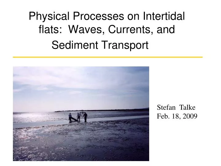
Physical Processes on Intertidal flats: Waves, Currents, and Sediment Transport . Stefan Talke Feb. 18, 2009. What is an Intertidal flat?. A muddy or sandy area without vegetation, generally in an estuary, which is exposed to air during low tide and covered by water during high tide. .

E N D
Physical Processes on Intertidal flats: Waves, Currents, and Sediment Transport Stefan Talke Feb. 18, 2009
What is an Intertidal flat? • A muddy or sandy area without vegetation, generally in an estuary, which is exposed to air during low tide and covered by water during high tide. San Francisco San Francisco Low Tide High Tide
Why do we care? • Estuarine boundary condition • Important for modeling estuarine physics correctly • Shoreline storm buffer (absorbs energy) • Source and sink of sediments, contaminants • Transfer to/from deeper waters (e.g., shipping channels) • Pollution often buried in mudflats • Mercury and other heavy metals, PCB’s, hydrocarbons, pesticides, etc. buried in the San Francisco Bay • Ecologically important • Intertidal flats very productive • Benthic diatoms account for 50% of primary production in Ems estuary, The Netherlands (de Jonge) • Nursery for juvenile (small) fish, invertebrates (protected from predation) • Clams, oysters, worms, shrimp live in mud Benthic diatoms Photos from V. de Jonge
N 0 200 m Experiment Location: San Francisco Bay Location of Experiment x Heavy metal pollution Research question: What governs fate of contaminated sediment?
Theoretical Preliminaries Sediments Contaminants Nutrients/Biota Settling Turbulence Bedload Transport Question: How can one understand the fate and transport of contaminants? MHHW ~2 m Marsh MLLW Worms Amphipods Clams
Theoretical Preliminaries Our approach: Focus on sediment transport budget MHHW Flux ~2 m Marsh MLLW Erosion – Deposition = Flux offshore Flux offshore = mass per unit time = sum of u * C over water column (dispersion neglected) u = horizontal velocity C = suspended sediment concentration Basically accounting—if you know u(z) and C(z), can predict evolution of tidal flat easy, right?
Multiple velocity, turbidity, and salinity sensors Deployed autonomously for days to weeks Experimental Setup Conductivity Temperature Depth probes Acoustic Doppler Velocimeters Optical Backscatter
Stratification • Stratification significant • >0.5 kg/ m3 between 10 cm and 50 cm depth • Fluctuations at seiche frequency during ebb
7 hours 70 minutes 60 seconds 60 seconds Velocity Data Observation: Many time scales of variability
(~0.002 Hz) ~0.1 Hz ~ 0.5 Hz Power Spectrum • Multiple frequencies of motion present over a tidal period <0.0001 Hz
Wind data correlation Only onshore directed wind considered Experiment N Wind from south Correlation wind/wave energy Significant correlation for f > 0.3 Hz Conclusion: The highest frequency of variation occurs due to local wind waves
Comparison of buoy wave spectrum and mudflat power spectrum Mudflat power spectrum Ocean buoy wave spectrum
Typical direction of ocean swell Refraction Bathymetrical Map of San Francisco Bay X marks experiment site X X Reflection? Bathymetry makes it unlikely for ocean swell to reach mudflat—yet they do!
X marks experiment site = Seiching Forcing 2-3.5 m ~ 2-3 km Lower frequency seiching Bathtub Analogy X X • Forcing = wind, perhaps tide • When forcing stops, sloshing begins Wave Speed = sqrt ( g* H) Wave period ~ 250-700 seconds
What drives suspended sediment concentrations? • Not tidal velocities (exert too little stress) • Often, local wind waves • But not always
Unidirectional flow Unlikely… ? What drives suspended sediment concentrations? • Seiching produces anomolous response Reversal of flow due to wave action Bedload Transport: Settling on lee side of ripples Vortex eats at lee side of ripple, ejects sediment into water column
Velocity Reversals Tide 5 • During positive seiching motion, frequency of velocity reversal is much greater • Why?
Comparison of waves • Tide 5: Ocean swell dominated • --As depth decreases, goes non-linear • -- concentration fluctuations at ocean swell frequency • Tide 8: Wind wave dominated • -- Are not nonlinear over measured depths Tide 8 Concentration Concentration Velocity Tide 5 Velocity
What drives suspended sediment concentrations? • Large gradients in salinity ‘trap’ sediment in fronts • Not directly related to wind waves or seiching • Called the ‘turbid tidal edge’
What drives suspended sediment concentrations? • Large gradients in salinity ‘trap’ sediment in fronts • Not directly related to wind waves or seiching • Called the ‘turbid tidal edge’
Definitions • Separate raw velocity and concentration data into following frequency bands • --Wave: 0.5 sec < T<100 sec • --Seiche: 100 sec< 1500 sec • --Tidal: T> 1500 sec • Question: What are the implications of multiple frequencies of motion to sediment erosion, deposition, and transport? Flux: Sediment Fluxes Positive Transport Direction
Tidally averaged sediment fluxes Flow rate near bed (~ 10 cm) Effect of freshwater discharge, storm surge Suspended sediment concentration near bed (~ 10 cm) Storm period tides 1-4
Tidally varying sediment fluxes Velocity Thought experiment: symmetric conditions + shorewards time Suspended sediment concentration (SSC) time What is the net flux (uC) over the tidal (wave) period? (none)
Tidally varying sediment fluxes Velocity Slightly different case: Asymmetric SSC + shorewards time Suspended sediment concentration (SSC) time (towards the shore) What is the net flux (uC) over the tidal (wave) period?
Tidally varying sediment fluxes Velocity + shorewards Third thought experiment: Asymmetric velocity time Suspended sediment concentration (SSC) time What is the net flux (uC) over the tidal (wave) period? (offshore)
Tidally varying sediment fluxes Conclusion: Asymmetries in velocity and/or SSC drive sediment fluxes over a tidal (or wave) period Here, we construct symmetric functions to determine whether SSC or velocity variation drives transport
Tidally varying sediment fluxes During storm (tides 1-4), asymmetries in tidal velocity and SSC drive fluxes After storm (tides 5-8), asymmetries in only SSC drive fluxes
Total sediment fluxes Big difference in magnitude, direction, and cause of sediment fluxes between storm and non-storm periods
Longer View Wave forcing inherently over only a portion of a tide Tidally varying fluxes ubiquitous
Longer View Long term bias towards large events occurring during the flood tide Time (hrs*12) Day of year
Summary of Hydrodynamic forcing Near-bed flow characterized by following motions: • Tidal Motions (T ~ 12 hours) • Large changes in depth (0 -1.5 m) • Spring-Neap variation • Ebb Dominated • Seiching Motions (T~ 500 seconds) • Seiche in the Inner Richmond Harbor, most likely due to wind wave setup or asymmetric tidal phasing • Ocean Swell (T ~ 8-15 seconds) • Varies on time scale of days • Follows Rayleigh Distribution • Wind Waves (T ~ 1-3 seconds) • Extremely energetic events with timescale of hours or several days • Correlates with local winds and storm events
Summary of SSC Sediments are observed in water due to • Wind waves and ocean swell forcing • Seiching Motions (T~ 500 seconds) • Turbid tidal edge (frontal convergence process)
Conclusions • Tidally averaged fluxes due to order of magnitude increase in u and C occur during stormy periods • Freshwater forcing important • Asymmetry in C over tidal period dominates sediment fluxes in non-stormy periods • Elevated C observed due to waves, frontal processes, or seiching motions. These processes drive asymmetry during non-storm periods.
Conclusions • Estuaries have many of the physical characteristics of lakes • Semi-enclosed bodies of water lead to seiching (‘bath tub sloshing’) • Locally driven wind waves important • However, wave climate also analogous to open shore beach • Tides • Ocean swell, but scaled by smaller magnitudes and less violent forces • Intersection of these paradigms and time scales creates unique, challenging environment
Conclusions • Intertidal Environment dominated by asymmetry and nonlinearity • Asymmetry • Tides • Wave forcing (e.g., Wind waves) • Ripples • Sediment concentration • Non-linearity • Waves (ocean swell) • Interaction between waves and currents
Ocean Swell Erosion: & velocity reversals Sediments Contaminants Nutrients/Biota Settling Updated view of Intertidal Mudflat Other processes? Tidal Forcing Stratification Wind Waves Seiche MHHW ~2 ft Marsh MLLW Worms Bedload Transport + sediment pumping Amphipods Clams Turbulence
Thanks to an NIEHS project for support , and many colleagues for field assistance