Download

1 / 16
190 likes | 294 Views
Pipeline Corrosion R&D at NIST. Richard E. Ricker Metallurgy Division Materials Performance Group Materials Science and Engineering Laboratory National Institute of Standards and Technology US Dept. of Commerce, Tech. Admin. Gaithersburg, MD 20899-8553 richard.ricker@nist.gov. Objective:.

E N D
Pipeline Corrosion R&D at NIST Richard E. Ricker Metallurgy Division Materials Performance Group Materials Science and Engineering Laboratory National Institute of Standards and Technology US Dept. of Commerce, Tech. Admin. Gaithersburg, MD 20899-8553 richard.ricker@nist.gov
Objective: • Starting with the results of original NBS burial studies for bare pipe in different soils; • (1) Analyze the data (new look, techniques, angles) • (2) Look for previously unrevealed relationships (new meaning) • (3) Identify R&D needs (gap analysis) • (4) Identify a path forward (experiments) • (5) Create understanding (results) • (6) Implement change(impact) • Why? • Because the bare pipe corrosion rate model underpins regulatory and repair decision making.
Objective:Review NBS Underground corrosion studies 1910-1957 Phases of Program 1. 1910: Congress authorized stray current corrosion study 2. 1920: Workshop convened to plan an underground corrosion study a) Dept of Agriculture selects sites b) Industry identifies and provide materials c) Symposia held every 5 years 4. 1922: Ferrous pipe materials at 47 sites for 12 to 17 years 5. 1924: Other materials buried at the sites during first retrieval 6. 1928: Fe alloys, Cu, Cu alloys, and Pb samples buried at new sites 6. 1932: Materials for corrosive soils study using 15 sites (coatings) 7. 1937, 1941, 1947 materials added during retrievals at the 15 sites 8. 1945: “Underground Corrosion” by K. H. Logan NBS C450 9. 1952: Last retrival - 128 sites, >36,000 samples, 333 matl types 10. 1957: Final Rpt. “Underground Corrosion” by M. Romanoff NBS C589 11. A larger number of follow-on studies from 1957 to the present: Ductile Cast Iron, Concentric Neutrals, Steel Pilings, Offshore Pilings, Stainless Steels, Bridge Deck Corrosion, etc.
Conclusions of Old NBS Studies • Some soils are very corrosive to bare pipe • Some soils are not very corrosive to bare pipe • Localized attack (pitting) is a problem in some soils • Large scatter was observed • All ferrous materials corroded at about the same rates (well within the measurement scatter) • Considerably less corrosion was observed in piles driven into undisturbed soil than in this study with disturbed (aerated) soils. • Clearly three factors stand out: • Aeration (disturbed vs. undisturbed), • Drainage (water in contact with surface), • High statistical variation in local occlusion cells • Conductivity indicates total salt content, and • Conductivity is only a rough indicator of soil corrosivity.
Original AnalysisAnalysis of Corrosion Kinetics Regression analysis for relationship of the form D=ktn The original NBS analysis determined an average k and n for each of the 47 soils. These were determine by linear regression of the equation Log (D) = Log (k) + n Log (t) Multiple linear regression of the k and n values as a function of soil properties met with only moderate success
Kinetic Analysis Bare surface with mixing P=kt Surface film slows transport P=ktn n=1/2, 1/3, 1/4 Reactant consumed from environment P=k[1-exp(-t/b)] Therefore, the slope n is an indicator of the rate determining (limiting) process Two rates: (i) corrosion rate, and (ii) the penetration (pitting) rate The pitting factor (PF) is the ratio of these two rates
Analysis of the maximum pit depth data indicates that pits grow at a rate that decreases with exposure time. For maximum pit depths, the exponent varied from about 1/4 to 1/2. Analysis of the mass lost data indicates a higher exponent or mixed rate determining kinetics (e.g. pitting and uniform attack) Multiple regression analysis for environmental factors influencing the exponent n has not yielded strong indicators. Understanding the scatter in the data should help analysis. Results of Kinetic Analysis
Statistical Analysis of ScatterExtreme Value Statistics Fundamental and Extreme Value Distributions Fundamental Distributions
Kinetic Models and Scatter Note, one assumes that the initial scatter is due to initiation times
Example Site Data Evidence for constant, increasing, and decreasing slopes were observed
Results of Extreme Value Analysis • Scatter consistent with different kinetic models were observed. • This may not be inconsistent with a decreasing rate model • The source of the scatter needs to be understood. • Variation in the environment • Alternating wet and dry • Salts in pit absorbing water Hypothesis 1 Hypothesis 2 Hypothesis 3
Gap Analysis and Path Forward Gap: Basic understanding of the origin of the observed scatter: (1) Pit initiation (2) Pit propagation (3) Environmental variations (annual, site, irregular) Path Forward Piggable and unpiggable pipes Laboratory Experiments designed to answer these questions
Experimental Evaluation Continuous Monitoring With Electrochemical Noise EIS of Sample Cut From Pipeline Steel Initial Focus: Rates in environments, range of rates, and transients Followup: Pit formation and propagation rate measurement.
Conclusions • Assuming that corrosion rates are determined by the alloy, environment, and the conditions of exposure, then the scatter observed in the original NBS study must be due to variations in one of these factors that was not quantified sufficiently. • Based on this analysis, and the findings of the original study, it was hypothesized that variations in ground water levels and sample wetting are the most probable explanations for the observed scatter. (other possibilities include variations in aeration, soil composition, and MIC) • Pitting rates were found to decrease with exposure time. This was also reported in the original study. The exponent determined for this behavior is close to that reported for pitting in the literature for aqueous environments. However, this knowledge cannot be used in a rate model until the source of the scatter is better understood. • If the origin of the scatter is understood and sufficient data for computer modeling of the rates is obtained, then prediction of the expected flaw growth rate and the expected range of rates for any particular environment and range of expected conditions should be possible. • The objective of the laboratory experiments is to identify the source of the scatter and obtain the information required for modeling of corrosion rates.