Download
1 / 17
170 likes | 325 Views
Global Monitoring of Tropospheric Pollution from Geostationary Orbit. Kelly Chance Harvard-Smithsonian Center for Astrophysics. Collaborators. Xiong Liu NASA/UMBC Thomas Kurosu Harvard-Smithsonian Center for Astrophysics The GeoTRACE Team:

E N D
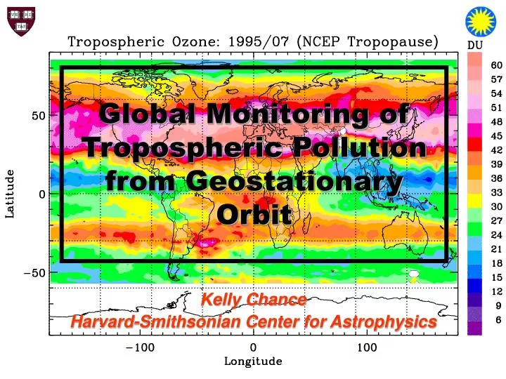
Global Monitoring of Tropospheric Pollution from Geostationary Orbit Kelly Chance Harvard-Smithsonian Center for Astrophysics
Collaborators Xiong Liu NASA/UMBC Thomas Kurosu Harvard-Smithsonian Center for Astrophysics The GeoTRACE Team: Jack Fishman, Doreen Neil, James Crawford (NASA); David Edwards (NCAR); Kelly Chance, Thomas Kurosu (Harvard-Smithsonian Center for Astrophysics); Xiong Liu (NASA/UMBC); R. Bradley Pierce (NOAA); Gary Foley, Rich Scheffe (EPA) AGU Spring Meeting
Outline • Introduction and motivation • NRC Decadal Survey: GeoCAPE Mission • Determination of measurement requirements • UV/visible gases discussed here • Gas concentrations • Geophysical, spatial, and temporal requirements • Scalable strawman • Future work – The two outstanding requirements AGU Spring Meeting
Introduction and Motivation • Target tropospheric gases are O3, NO2, SO2, HCHO, CHO-CHO (plus CO and O3 in IR, plus aerosols, not discussed here). • The aims are: • To retrieve tropospheric gases from geostationary orbit at high spatial and temporal resolution. • To integrate the results into air quality prediction, monitoring, and modeling, and climatological studies. • Experience from previous satellites: Scientific and operational measurements of O3, NO2, SO2, HCHO, and CHOCHO (and BrO, IO, OClO, H2O). AGU Spring Meeting
Fitting trace species • Requires precise (dynamic) wavelength (and often slit function) calibration, Ring effect correction, undersampling correction, and proper choices of reference spectra (HITRAN!) • Remaining developments: • Tuning PBL O3 from UV/IR combination (demonstrated for the OMI/TES combination by SAO/UMBC + JPL) • Tuning direct GOME/SCIAMACHY PBL SO2 from optimal estimation (underway @ SAO/UMBC/U. Toronto)
Required Concentrations* *In PBL. Determined from our satellite measurements. (Future: traceability from AQ requirements and modeling)
Geostationary Minimal Case:Scalable Strawman - 1 15o - 50o N, 60o - 130o W (parked at 0o N, 95o W) Measure solar zenith angles from 0o – 70o
Radiative Transfer Modeling and Fitting Studies Note cloud windows: Use of Raman scattering and of the oxygen collision complex. O2A band
Measurement RequirementsTo Meet Required Concentrations The slant column measurement requirements come from full multiple scattering calculations, including gas loading, aerosols, and the GOME-derived (Koelemeijer et al., 2003) albedo database, and assume a 1 km boundary layer height.
Scalable Strawman - 2 Lat/lon limits are ~3892 km N/S and 7815-5003 km E/W (6565 average), or about 390657 1010 km2 footprints. • Measure 400 spectra N/S in two 200-spectrum integrations (each on two 10242 detector arrays – 1 UV and 1 visible). • 2.5 seconds per longitude (21 s integration, 0.5 s step and flyback) total sampling every < ½ hour (27 min). Detectors: Rockwell HyViSi TCM8050A CMOS/Si PIN • 3106 e- well depth; will need several rows (or readouts) per spectrum to reach the necessary statistical noise levels. • Complicated by brightness issues; can’t always have full wells.
Scalable Strawman - 3 • 200 spectra on each of two 10242 arrays; each spectrum uses 4 detector rows (800 total out of 1024). • Channel 1: 280-370 nm @ 0.09 nm sample, 0.36 nm resolution (FWHM). • Channel 2: 390-490 nm @ 0.1 nm sample, 0.4 nm resolution (FWHM); includes O2-O2 @ 477 nm. • Nyquist sampled: 4 samples per FWHM virtually eliminates undersampling for a symmetric instrument transfer (slit) function [Chance et al., 2005]. • Pointing to 1 km = 1/35,800 = 6 arc second (easy). • Size optics to fill sufficiently in 1 second ( 1 cm2 (GOME size) √1.5 (GOME integration time) 35,800 km / 800 km = 55 cm “telescope” optics). More realistically ….
Sizing for 1010 km2 Footprint,1 Second Integration Time • Rad: Minimum clear-sky radiance, cross-section weighted (photons s-1 nm-1 sr-1 cm-2) • cm-2 px-1: # photons cm-2 pixel-1 @ instrument in 1 second; 1010 km27.80 10-8 sr solid angle • RMS: Fitting RMS required for the minimum detectable amount = 1 / required S/N • px-1: # photons pixel-1 needed in 1 second to meet RMS-S/N requirements; includes factor of 4 for 4 detectors rows per spectrum • aEff: Telescope collecting area (cm2) overall optical efficiency
Sizing for 1010 km2 Footprint,1 Second Integration Time Formaldehyde (HCHO) is the driver for almost any conceivable choice of requirements! (Unless VOCs are considered unimportant, in which case O3 would be the driver, with the above as a low estimate). 20.76 cm2 is a16-cm diameter telescope @ 10% optical efficiency (GOME, a much simpler instrument, is 15 – 20% efficient in this wavelength range). Also, IR needs (CO, O3) plus aerosols must be addressed.
Major Tradeoffs and Questions Tradeoffs: # samples (footprint) vs. sensitivity (S/N) vs. integration time vs. geographical coverage vs. max SZA: • 55 km2 footprints in 1/2 hour with a 32 cm diameter telescope, if the instrument is 10% efficient. Questions: Are lat and lon sampling necessarily the same? Is constant sampling necessary? Option: MODIS channels for aerosols? (TOMS absorbing aerosol index is automatic, but little else operationally.) • OMI aerosol products should be reviewed. • Should include polarization-resolved measurements; • Several such UV channels will improve PBL O3 [Hasekamp and Landgraf, 2002a,b; Jiang et al., 2003]. Everything is debatable; this is why it is a strawman, but we must show why alternatives are better.
Outstanding Needs • Science Requirements (S/N, geophysical, spatial, temporal) from sensitivity and modeling studies (OSSEs), providing traceability for AQ forecast improvement and other uses. • Unless things change a lot, HCHO will be the driver for instrument requirements. Then address trade space. • Instrument Design. Reducing “smile”, enabling multiple readouts, increasing efficiency, optimizing ITF shape …. • GEO instrument is not just a super-OMI with CMOS/Si detectors instead of CCDs. Minimal geostationary requirements imply scanning instead of a pushbroom and they imply getting many more spectra onto a rectangular detector than OMI has obtained. • Instrument optical and spectrograph design is the single most important outstanding issue in demon-strating the feasibility of geostationary pollution measurements.