Download
1 / 13

E N D
The large scale econometric models The first large-scale econometric model was built by Professor Lawrence Klein in the 1950s. The equations which formed the model represented a “synthetic” or artificial economy.The modelwent through various iterations and evolved into the MIT-FR-Wharton model
Uses of the model • Using this model, it was possible to simulate the effects of proposed fiscal policy measures such as increased military spending and tax cuts on a wide array of aggregate (Y, I, C, S, ...) and disaggregate level variables (truck sales, employment in construction trades, cement prices). • For example, The people who ran the model were asked to simulate the impact of the proposed Kennedy-Johnson tax cuts in the early 60s (took effect in 1964) on a broad array of economic variables.
A simple macro model Consider the following economy: Yt = Ct + It + Gt + Xt – Mt [5.5] Equation [5.5] can be read as follows: Total output in period t is equal to total spending for new goods and services in period t , or consumption plus investment plus government expenditure plus imports minus exports. Equation [5.5] is an identity—that is, it is true by definition
The behavioral equations Ct = a + b(Yt – Tt) + dPt – 1 [5.6] Tt = e + fYt [5.7] It = h + jYt – 1 + kRt [5.8] Mt = n + qYt [5.9] Pt = s + uYt + vPt – 1 [5.10] We call these behavioral equations because they describe the way the way the spending category has behaved in the past as a function of the explanatory variables.
Finding the reduced form First, we substitute the behavioral equations [5.6] through [5.10] into [5.5] to obtain the following (we have dropped the t subscripts to economize on notation): Y = [a + b(Y – e – fY) + dPt – 1] + (h + jYt-1 + kR) + G + X – (n + qY) By rearranging this equation, we obtain the following reduced form equation [5.11]
Exogenous and endogenous variables • Exogenous variables are determined outside the model. They may be know by forecasters—or forecasters may have to forecast them In our model: X, G, and R • Endogenous variables are determined within the model—specifically, by equation [5.11] In our model: Y, C, I, T, M, and P
Forecasting using the reduced form • The forecaster can estimate the values of a, b, d, e, f, h, j, k, n, q, s, u, and v with time series regression analysis. • Pt – 1 and Yt – 1 are known • That leaves the exogenous variables Gt, Xt, and Rt. Perhaps Gt is known. The forecaster will have to estimate (forecast) the values of the other exogenous variables
The Suits modela The article is noteworthybecause is educatedeconomists on the newapplications of econometrics made possible by advances in computer technology Y = C + I + G (1) C = 20 + 0.7(Y - T) (2) I = 2 + .01Yt - 1 (3) T = 0.2Y (4) • The unkown variables are Y, C, I, and T • The known variables are G and Yt - 1. aDaniel Suits.” Forecasting and Analysis with an Econometric Model,” American Economic Review, March 1962: 104-132.
A simple national econometric model a Consider a closed economy with government GDP = C + I + G GDP is the dependent variable.Hence, to get solution for GDP, we mustfirst specify and estimate models for C, I, and G a The following is based on A. Migliario. “The National Econometric Model: A Layman’s Guide,” Graceway Publishing, 1987.
The aggregate level specifications GDP t + 1 = C t + 1 + I t + 1 + G t + 1 (2) C t + 1 = 1 + 2DYt + et (3) I t + 1 = 3 + 4it + et (4) G t + 1 = 5 + 6Gtb (5) • Migliaro used OLS to estimated 1, 2, 3, 4, 5, and 6 • Having accomplished that, he substituted estimated equations (3), (4), and (5) back into (2) to get a forecasted value of G t + 1. • An example: I t + 1 = 11.567 - 0.419it b Migliaro used the trend component to forecast G.
Extending (disaggregating) the model Let: C t + 1 = DUR t + 1 + NONDUR t + 1 + SERVICES t + 1 Now let: DUR t + 1 = AUTOS t + 1 + FURNITURE t + 1 + APPLIANCES t + 1 + . . . Now let:AUTOS t + 1 = Passenger Cars t + 1 + Vans t + 1 + Trucks t + 1 + . . .
A trucks specification Trucks t + 1 = 1 + 2DYt + 3AGEt + 4PRICEt + et • As we increase the level of disaggregation, we increase the number of equations.That is, we could have equations for different classes of trucks--midsize, etc. • It is the disaggregate level forecasts which are most valuable tobusiness decision-makers. • Entities such as DRI-McGraw Hill and Chase econometrics sell disaggregate-level forecasts to a high-powered client base.
A lot of equations • The DRI-McGraw Hill Model has approximately 450 equations. • The FRB-MIT-Wharton model has 669 equations. • The Chase Econometrics modle has 350 equations • The Kent model has 44,400 equations.