Download
1 / 15
150 likes | 266 Views
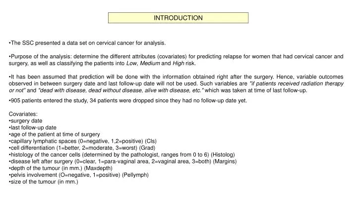
INTRODUCTION. The SSC presented a data set on cervical cancer for analysis. Purpose of the analysis: determine the different attributes (covariates) for predicting relapse for women that had cervical cancer and surgery, as well as classifying the patients into Low , Medium and High risk.

E N D
INTRODUCTION • The SSC presented a data set on cervical cancer for analysis. • Purpose of the analysis: determine the different attributes (covariates) for predicting relapse for women that had cervical cancer and surgery, as well as classifying the patients into Low, Medium and High risk. • It has been assumed that prediction will be done with the information obtained right after the surgery. Hence, variable outcomes observed in between surgery date and last follow-up date will not be used. Such variables are "if patients received radiation therapy or not” and "dead with disease, dead without disease, alive with disease, etc." which was taken at time of last follow-up. • 905 patients entered the study, 34 patients were dropped since they had no follow-up date yet. • Covariates: • surgery date • last follow-up date • age of the patient at time of surgery • capillary lymphatic spaces (0=negative, 1,2=positive) (Cls) • cell differentiation (1=better, 2=moderate, 3=worst) (Grad) • histology of the cancer cells (determined by the pathologist, ranges from 0 to 6) (Histolog) • disease left after surgery (0=clear, 1=para-vaginal area, 2=vaginal area, 3=both) (Margins) • depth of the tumour (in mm.) (Maxdepth) • pelvis involvement (O=negative, 1=positive) (Pellymph) • size of the tumour (in mm.)
EXPLORATORY ANALYSIS Univariate plots by variables, such as these, were performed to better understand their behaviour. Also pairwise contingency tables were used as an exploratory tool.
EXPLORATORY ANALYSIS Classification trees are used to uncover inherent structure in data. These are binary arrangements created by splitting observations into “more homogeneous” groups, dictated by rules of the form:(e.g.) “if Age<24 and Cls is positive then response is likely 1” Misclassification Rate= .06774Residual Mean Deviance= 0.2995 When dropping observations with NA,too much information is lost, will use NA’s as a factor in all variables. Complex model, a smaller tree might do...
EXPLORATORY ANALYSIS Just as regression uses Residual Sum of Squares as a diagnostic of fit, trees use Residual Deviance. Hence a decrease in deviance means a better fitted tree. In regression, more parameters might give a better fit but complex interpretation. Here, number of terminal nodes is analogous to the latter. Pruning of a tree can be done based on the following: Misclassification Rate= .07233Residual Mean Deviance= 0.3696 This smaller tree is easier to follow and the misclassification ratio is still of acceptable size. Maxdepth, Size and Cls are observed to be important variables in the structure.
Proportional Hazards Assumption was not violated neither individually nor as a global model (pvalue=0.14) • Variable Size is of importance as seen in trees. Nevertheless, it has many missing values, and analyses usually drop such observations. In order to keep information we categorised it with the missing values as the lowest of the levels and used the quartiles as cutoffs for the other levels. SURVIVAL ANALYSIS A Cox Proportional Hazards model was assumed. During the process of modeling, it was seen that the important levels of Size were three categories: Not Measured (NA’s), 30 and >30 The model for prediction agreed on included Age, Cls, Maxdepth and Size as predictors, along with two two-way interactions: Age with Cls and Maxdepth with Size. Specifically the hazard as a function of time can be seen as
SURVIVAL ANALYSIS The Cox curves were calculated as the average of the curves corresponding to the different covariate patterns, rather than plotting curves with the average VALUE of the covariates. (used S-plus function avg.surv created by Dr. R. Brant, CHS Dept, U of C )
SURVIVAL ANALYSIS • Some interesting results and interpretation for the model: • The hazard ratio for comparison between having Cls positive1 to positive2, keeping all other variables fixed: Similarly, we can look at hazard ratio for an increase in tumour size, mainly: So, for Age=30, the hazard ratio=4.166265, that is, the hazard of having a relapse when Cls positive1 is 4.16625 times greater than the hazard of relapse when Cls positive2 at age 30 Now, for Age=50 hazard ratio=0.2963008 With analogous interpretation. We can see the effect of the interaction between Age and Cls So, for Maxdepth=10, hazard ratio=0.59097, that is, the hazard of having a relapse when Size is less than 30 is .2963008 times the hazard of relapse when Size>30. • As with any model, assumptions are needed. The assumption of non-informative censored data (censoring not related to the chances of recurrence) was used.
LOGISTIC REGRESSION ANALYSIS • The main model for a Logistic regression is to regress the log of the odds of a binary output event as a linear function of covariates. • Odds is the ratio of the probability of an event happening and the probability of the same event not happening Recall that during the process of modeling, it was seen that important levels of Size were really three categories: Not Measured (NA’s), 30 and >30 The model for prediction agreed on included Age, Cls, Maxdepth, Size and Pellymph as predictors, along with a two-way interaction between Age and Cls. Specifically the logistic model can be seen as The statistical significant model included an interaction between Pellymph and Size >30. However, there were only three observations with such values and the inclusion of this interaction created problems for prediction. Hence, for the sake of interpretability and in order to be able to predict, we decided to drop it. The change in residual deviance from the fuller model to the one kept was from 252.99 to 260.99.
LOGISTIC REGRESSION ANALYSIS The usual plot for this type of analysis is a probability curve. Given the fact that we had 2 continuous variables in our model, we present some examples of probability surfaces. This enables to look for any Age/Maxdepth combination Observe interaction of Age and cls
LOGISTIC REGRESSION ANALYSIS We can see that Age plays a bigger role when Cls has level of positive2 Changing from Size <=30 to Size >30 increments the probability of relapse, for a fixed set of the other variables (compare top to bottom)
LOGISTIC REGRESSION ANALYSIS • Some interesting results and interpretation for the model: • The odds ratio for comparison between having Cls positive1 to positive2, keeping all other variables fixed: Similarly, we can look at odds ratio for an increase of 10mm in tumour depth, mainly: So, for Age=30, the odds ratio=3.190795, that is, the odds of having a relapse when Cls positive1 are 3.190795 times greater than the odds of relapse when Cls positive2. Now, for Age=50, the odds ratio=0.2602293, with analogous interpretation. We can see the effect of the interaction between Age and Cls So, for fixed values of other variables, and an increase in 10 for Maxdepth, the odds ratio=1.935962. That is, the odds of having a relapse when tumour is 10mm deeper are 1.935962 times greater.
LOGISTIC REGRESSION ANALYSIS Classified + if predicted Pr(D) >= .5 -------- True -------- Classified | D ~D Total - ----------+--------------------------+----------- + | 5 3 | 8 - | 37 612 | 649 ---------+--------------------------+----------- Total | 42 615 | 657 True D defined as relapse ~= 0 Positive predictive value Pr( D| +) 62.50% Negative predictive value Pr(~D| -) 94.30% Correctly classified 93.91% One of the purposes of the case study was to classify patients in Low, Medium and High risk of relapse. We suggest to do this using the probabilities obtained from this logistic regression in the following way: Calculate the probability from the model for each patient. If the probability is within a prefixed range, then it is set as Low, if it is within another range Medium and so on. For example : Low if in (0,.35], Med if in (.35, .60] and High if >.60 Another way for classifying, would involve at risk or not at risk as the possible classifications (as a +/- test). Although this gives only two possibilities, predictive values can be calculated and hence have a measure of accuracy. Do this by setting a cutoff point for the probabilities calculated and set the value of the test for the patient as + or -. Some examples for different cutoffs follow. • For the next cutoff values the table itself is omitted.
LOGISTIC REGRESSION ANALYSIS As a “goodness of fit” , a table for groups follows Classified + if predicted Pr(D) >= .25 True D defined as relapse ~= 0 Positive predictive value Pr( D| +) 33.33% Negative predictive value Pr(~D| -) 94.76% Correctly classified 92.24% Logistic model for relapse, goodness-of-fit test (Table collapsed on quantiles of estimated probabilities) Group Prob Obs_1 Exp_1 Obs_0 Exp_0 Total 1 0.0150 1 0.8 65 65.2 66 2 0.0188 1 1.1 65 64.9 66 3 0.0216 0 1.3 66 64.7 66 4 0.0259 3 1.5 62 63.5 65 5 0.0318 2 1.9 64 64.1 66 6 0.0440 1 2.5 65 63.5 66 7 0.0604 4 3.4 61 61.6 65 8 0.0839 2 4.7 64 61.3 66 9 0.1413 12 6.9 54 59.1 66 10 0.6601 16 17.8 49 47.2 65 number of observations = 657 number of groups = 10 Pvalue= 0.2704 Classified + if predicted Pr(D) >= .4 True D defined as relapse ~= 0 Positive predictive value Pr( D| +) 70.00% Negative predictive value Pr(~D| -) 94.59% Correctly classified 94.22% Classified + if predicted Pr(D) >= .6 True D defined as relapse ~= 0 Positive predictive value Pr( D| +) 50.00% Negative predictive value Pr(~D| -) 93.74% Correctly classified 93.61%
CONCLUSIONS FUTURE WORK • Given the nature of the study, and the assumption that prediction of relapse would be done right after surgery, variables observed after surgery were not taken into account . These were: Status of patient at last follow-up date and if patients received radiation. • Contrary to what we expected, Disease left after surgery did not play an important role in prediction. • There was agreement throughout the different analyses (exploratory, survival and logistic) regarding the importance of the inclusion of three covariates: Maxdepth,Capillary Lymphatic Spaces (Cls) and Size. • The effect of variable Age on relapse is affected by its interaction with Capillary Lymphatic Spaces (cls) • The important variables for predicting the survival to relapse are Age, Cls, Size and Maxdepth. • The important variables for predicting the probability of relapse are Age, Cls, Size, Maxdepth and Pellymph. • It would be of relevance to check the importance of covariates when separating the response variable as no relapse, relapse before a specific time and relapse after that time. • Use of trees as a classification tool rather than an exploratory tool.
AKNOWLEDGEMENTS BIBLIOGRAPHY We would like to thank the following for their help and support in the creation of this poster: StatCar lab, Mathematics and Statistics Dept., U of C Dr. R. Brant, CHS, U of C Dr. P. Ehlers, Math and Stats, U of C B. Teare, Math and Stats, U of C Learning Commons, U of C • Rose, S., Lecture notes for Biostatistics II • Venables, W.N. and Ripley, B.D. Modern Applied Statistics with S-plus, Springer Statistics and Computing Series, New York, 1994 • Insightful, S-plus 2000 Guide to Statistics, Seattle, 1999