Download

1 / 51
550 likes | 822 Views
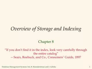
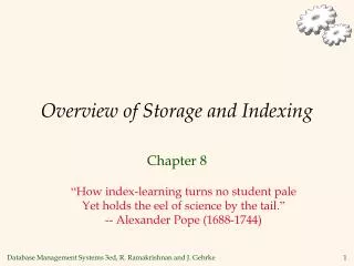
Overview of Storage and Indexing. Chapter 8. “How index-learning turns no student pale Yet holds the eel of science by the tail.” -- Alexander Pope (1688-1744). Why Concerning Storage and Indexing? . DB design using logical models (ER/Relational).

E N D
Overview of Storage and Indexing Chapter 8 “How index-learning turns no student pale Yet holds the eel of science by the tail.” -- Alexander Pope (1688-1744)
Why Concerning Storage and Indexing? • DB design using logical models (ER/Relational). • Appropriate level for designers to begin with • Provide independence from implementation details • Performance: another major factor in user satisfaction • Depends on • Efficient data structures for data representation • Efficiency of system operation on those structures • Disks contains data files and system files including dictionary and index files • Disk access: one of the most critical factor in performance.
Subjects to be Discussed • Disks: Can retrieve random page, but reading several consecutive pages is much cheaper than reading them in random order • Buffer manager: Stages pages from external storage to main memory buffer pool. File and index layers make calls to the buffer manager. • File organization: Method of arranging a file of records on external storage. • Record id (rid) is sufficient to physically locate record • Indexes are data structures that allow us to find the record ids of records with given values in index search key fields
Storage Hierarchy • DBMS stores information on some storage medium • Primary storage: can be operated directly by CPU. • Secondary storage: • larger capacity, lower cost, slower access • cannot be operated directly by CPU – must be copied to primary storage • Secondary storage has major implications for DBMS design • READ:transfer data to main memory • WRITE:transfer data from main memory. • Both transfers are high-cost operations, relative to in-memory operations, so must be planned carefully
Why Not Store Everything in Main Memory? • Cost and size • Main memory is volatile:What’s the problem? • Typical storage hierarchy: • Factors: access speed, cost per unit, reliability • Cache and main memory (RAM) for currently used data: fast but costly • Flash memory: limited number of writes (and slow), non-volatile, disk-substitute in embedded systems • Disk for the main database (secondary storage). • Tapes for archiving older versions of the data (tertiary storage).
Disks • Secondary storage device of choice. • Data is stored and retrieved in units called disk blocks or pages. • Unlike RAM, time to retrieve a disk page varies depending upon location on disk. • Therefore, relative placement of pages on disk has major impact on DBMS performance!
Tracks Arm movement Arm assembly Components of a Disk Spindle Disk head • The platters spin • The arm assembly is moved in or out to position a head on a desired track. Tracks under heads make a cylinder(imaginary!). Sector Platters • Only one head reads/writes at any one time. • Block size is a multiple of sector size (which is fixed).
Accessing a Disk Page • Time to access (read/write) a disk block: • seek time (moving arms to position disk head on track) • rotational delay (waiting for block to rotate under head) • transfer time (actually moving data to/from disk surface) • Seek time and rotational delay dominate. • Seek time varies from about 1 to 20msec • Rotational delay varies from 0 to 10msec • Transfer rate is less than 1msec per 4KB page • Key to lower I/O cost: reduce seek/rotation delays
Arranging Pages on Disk • `Next’ block concept: • blocks on same track, followed by • blocks on same cylinder, followed by • blocks on adjacent cylinder • Blocks in a file should be arranged sequentially on disk (by `next’), to minimize seek and rotational delay. • For a sequential scan, pre-fetchingseveral pages at a time is a big win!
Tracks Arm movement Arm assembly Spindle Disk head Sector Platters
RAID • Redundant Arrays of Independent Disks • Disk Array: Arrangement of several disks that gives abstraction of a single, large disk. • Goals: Increase performance and reliability. • Two main techniques: parallelism and redundancy • Data striping: Data is partitioned; size of a partition is called the striping unit. Partitions are distributed over multiple disks. • Redundancy: More disks -> more failures. Redundant information allows reconstruction of data if a disk fails. • RAID levels: level 0 – level 6
Disk Space Management • Lowest layer of DBMS software manages space on disk. • Higher levels call upon this layer to: • allocate/de-allocate a page • read/write a page • Highly desirable that a request for a sequence of pages to be satisfied byallocating the pages sequentially on disk.
Query Optimization and Execution Relational Operators Files and Access Methods Buffer Management Disk Space Management DB Structure of a DBMS These layers must consider concurrency control and recovery • A typical DBMS has a layered architecture. • The figure does not show the concurrency control and recovery components. • This is one of several possible architectures; each system has its own variations.
DB Buffer Management in a DBMS Page Requests from Higher Levels • Data must be in RAM for DBMS to operate on it. • Table of <frame#, pageid> pairs is maintained. BUFFER POOL disk page free frame MAIN MEMORY DISK choice of frame dictated by replacement policy
When a Page is Requested ... • If requested page is not in pool: • Choose a frame for replacement • If frame is dirty, write it to disk • Read requested page into chosen frame • Pin the page and return its address. • If requests can be predicted (e.g., sequential scans) • pages can be pre-fetchedseveral pages at a time!
More on Buffer Management • Requestor of page must unpin it, and indicate whether page has been modified: • dirtybit is used for this. • Page in pool may be requested many times, • a pin count is used. A page is a candidate for replacement iff pin count = 0. • CC & Recovery may require additional I/O when a frame is chosen for replacement. Why?
Buffer Replacement Policy • Frame is chosen for replacement by a replacement policy: • Least-recently-used (LRU), Clock, MRU, etc. • Policy can have big impact on # of I/O’s; depends on the access pattern. • Sequential flooding:Nasty situation caused by LRU + repeated sequential scans. • # buffer frames < # pages in filemeans each page request causes an I/O. MRU much better in this situation (but not in all situations, of course).
DBMS vs. OS File System OS does disk space & buffer mgmt: why not let OS manage these tasks? • Differences in OS support: portability issues • Some limitations, e.g., files can’t span disks. • Buffer management in DBMS requires different abilities • pin a page in buffer pool, force a page to disk (important for implementing CC & recovery), • adjust replacement policy, and pre-fetch pages based on access patterns in typical DB operations.
File Organizations Several alternatives exist, each ideal for some situations, and not so good in others: • Heap (random order) files:Suitable when typical access is a file scan retrieving all records. • Sorted files:Best if records must be retrieved in some order, or only a `range’ of records is needed. • Indexed files: For efficient searching • Which organization is best? How can you tell?
Efficient Searching Additional structures to help searching • Associated with data files to search for records based on certain field (search key) values • For direct record locating without sequential search. • Indexes: Data structures to organize records via trees or hashing. • Like sorted files, they speed up searches for a subset of records • Updates are much faster than in sorted files.
Cost Model for Our Analysis We ignore CPU costs, for simplicity: • B: The number of data pages • R: Number of records per page • D: (Average) time to read or write disk page • Measuring number of page I/O’s ignores gains of pre-fetching blocks of pages; thus, even I/O cost is only approximated. • Average-case analysis; based on several simplistic assumptions. • Good enough to show the overall trends!
Assumptions used for Analysis • Single record insert and delete. • Heap Files: • Equality selection on key; exactly one match. • Insert always at end of file. • Sorted Files: • Files compacted after deletions. • Selections on sort field(s). • Hashed Files: • No overflow buckets, 80% page occupancy.
Cost of Operations • Several assumptions underlie these (rough) estimates!
Indexes • An index on a file speeds up selections on the search key fieldsfor the index. • Any subset of the fields of a relation can be the search key for an index on the relation. • Search key is not the same as key(minimal set of fields that uniquely identify a record in a relation). • An index contains a collection of data entries, and supports efficient retrieval of all data entries k*with a given key value k. • Given data entry k*, we can find record with key k quickly.
B+ Tree Indexes Non-leaf Pages Leaf Pages (Sorted by search key) • Leaf pages containdata entries, and are chained (prev & next) • Non-leaf pages have index entries; only used to direct searches: index entry P K P K P P K m 0 1 2 1 m 2
Example B+ Tree Note how data entries in leaf level are sorted Root 17 • Find 28*? 29*? All > 15* and < 30* • Insert/delete: Find data entry in leaf, then change it. Need to adjust parent sometimes. • And change sometimes bubbles up the tree Entries < 17 Entries >= 17 27 5 13 30 39* 2* 3* 5* 7* 8* 22* 24* 27* 29* 38* 33* 34* 14* 16*
Hash-Based Indexes • Good for equality selections. • Index is a collection of buckets. • Bucket = primary page plus zero or moreoverflow pages. • Buckets contain data entries. • Hashing functionh: h(r) = bucket in which (data entry for) record r belongs. h looks at the search key fields of r. • No need for “index entries” in this scheme.
Static Hashing • # primary pages fixed, allocated sequentially, never de-allocated; overflow pages if needed. • h(k) mod N = bucket to which data entry withkey k belongs. (N = # of buckets) 0 h(key) mod N 1 key h N-1 Primary bucket pages Overflow pages
Index • What is an index? • An index on a file speeds up selections on the search key fieldsusedfor the index. • Any subset of the fields of a relation can be the search key for an index on the relation? • Is search key the same as key(minimal set of fields that uniquely identify a record in a relation)? • An index contains a collection of data entries, and supports efficient retrieval of all data entries k*with a given key value k. • Given data entry k*, we can find records with key value k quickly.
Index file and Data File • Example: ``Find all students with gpa > 3.0’’ • If data is in sorted file, do binary search to find first such student, then scan to find others. • Cost of binary search can be quite high. • Idea: Create an `index’ file. Index File kN k2 k1 Data File Page N Page 3 Page 1 Page 2 Can do binary search on (smaller) index file!
Data Entry k*in Index • A data entry k* refers to the records stored in an index file with search key value k • What does it contain? • It contains enough information to locate data record with search key value k • Idea: • Efficiently search an index with search key value k to find the data entries • Use them to obtain the desired data records • For a given search key value k, will there be exactly 0 or 1 data record?
Alternatives for Data Entry k*in Index • In a data entry k* we can store: • Data record with key value k, or • <k, rid of data record with search key value k>, or • <k, list of rids of data records with search key k> • Choice of alternative for data entries is orthogonal to the indexing technique used to locate data entries with a given key value k. • Examples of indexing techniques: B+ trees, hash-based structures • Typically, index contains auxiliary information that directs searches to the desired data entries
Alternatives for Data Entries (Contd.) • Alternative 1: • If this is used, index structure is a file organization for data records (instead of a heap file or sorted file). • At most one index on a given collection of data records can use Alternative 1. Why? • Otherwise, data records are duplicated, leading to redundant storage and potential inconsistency.
Alternatives for Data Entries (Contd.) • Alternatives 2 and 3: • When are they better than Alternative 1? • Data entries typically much smaller than data records. So, they are better than Alternative 1 with large data records, especially if search keys are small. • Compare Alternatives 2 and 3 -- which one is better? • Alternative 3 is more compact than Alternative 2, but leads to variable sized data entries even if search keys are of fixed length.
Index Classification • Primary vs. secondary: If search key contains primary key, then called primary index. • Different defs in other books • Unique index: Search key contains a candidate key.
Dense vs Sparse Index • Dense index: one index entry per search key value. • Sparse index: index records for only some of the records • Every sparse index is clustered! • Sparse indexes are smaller • Which one is faster? • Which one has less overhead? Ashby, 25, 3000 22 Basu, 33, 4003 25 Bristow, 30, 2007 30 Ashby 33 Cass, 50, 5004 Cass Smith Daniels, 22, 6003 40 Jones, 40, 6003 44 44 Smith, 44, 3000 50 Tracy, 44, 5004 Sparse Index Dense Index on on Data File Name Age
Clustered Index • Clustered vs. unclustered: If order of data records is the same as, or `close to’, order of data entries, then called clustered index. • Alternative 1 implies clustered • Can a file be clustered on with more than one search key? • Can non-key field become clustering index? • Cost of retrieving data records through index varies greatly based on whether index is clustered or not. Why? • If the index is clustered, rids of qualifying data entries point to a contiguous collection of records, and we need to retrieve only a few data pages. • If unclustered, each qualifying data entry could contain a rid that points to a distinct data page, leading to I/O
Clustered vs. Unclustered Index • Suppose that Alternative (2) is used for data entries, and that the data records are stored in a Heap file. • To build clustered index, first sort the Heap file (with some free space on each page for future inserts). • Overflow pages may be needed for inserts. (Thus, order of data recs is `close to’, but not identical to, the sort order.) Index entries UNCLUSTERED CLUSTERED direct search for data entries Data entries Data entries (Index File) (Data file) Data Records Data Records
Understanding the Workload • Why necessary? • For each query in the workload: • Which relations does it access? • Which attributes are retrieved? • Which attributes are involved in selection/join conditions? How selective are these conditions likely to be? • For each update in the workload: • Which attributes are involved in selection/join conditions? How selective are these conditions likely to be? • The type of update (INSERT/DELETE/UPDATE), and the attributes that are affected.
Choice of Indexes • What indexes should we create? • Which relations should have indexes? • What field(s) should be the search key? • Should we build several indexes? • For each index, what kind of an index should it be? • Clustered or not? • Dense or sparse? • Hash/tree?
Choice of Indexes (Contd.) • One approach: Consider the most important queries in turn. Consider the best plan using the current indexes, and see if a better plan is possible with an additional index. If so, create it. • Before creating an index, must also consider the impact on updates in the workload! • Is there a trade-off for using index between updates and queries? • Trade-off: Indexes can make queries go faster, updates slower. Require disk space, too.
Index Selection Guidelines • Attributes in WHERE clause are candidates for index keys. • Exact match condition suggests hash index. • Range query suggests tree index. • Clustering is especially useful for range queries; can also help on equality queries if there are many duplicates. • Multi-attribute search keys should be considered when a WHERE clause contains several conditions. • Try to choose indexes that benefit as many queries as possible. • Since only one index can be clustered per relation, choose it based on important queries that would benefit the most from clustering.
Examples of Clustered Indexes SELECT E.dno FROM Emp E WHERE E.age>40 • Tree or hashing? • B+ tree index on E.age can be used to get qualifying tuples. • Things to consider: • How selective is the condition? • If 99% are over 40, is index useful? • If 10%, is an index useful? • Depends on whether the index is clustered • If unclustered, it can be more expensive than sequential scan with only 10%
Examples of Clustered Indexes • Consider the GROUP BY query: using age as an index ---- is it effective? • If many tuples have E.age > 20, using E.age index and sorting the retrieved tuples may be costly. • Especially bad if this index is not clsutered • Clustered E.dno index may be better! SELECT E.dno, COUNT (*) FROM Emp E WHERE E.age>20 GROUP BY E.dno
Examples of Clustered Indexes SELECT E.dno FROM Emp E WHERE E.hobby=Stamps • Clustering is important for an index on a search key that is not a candidate key • Equality queries and duplicates: • Clustering on E.hobby helps! • What if WHERE E.eid=554 instead of WHERE E.hobby=Stamps? • Does clustered index helpful in this case?
Indexes with Composite Search Keys Examples of composite key indexes using lexicographic order. • Composite Search Keys: Search on a combination of fields. • Equality query: Every field value is equal to a constant value. E.g. wrt <sal,age> index: • age=12 and sal =75 • Range query: Some field value is not a constant. E.g.: • age =12; or age=12 and sal > 10 • Data entries in index sorted by search key to support range queries. 11,80 11 12 12,10 name age sal 12,20 12 13,75 bob 12 10 13 <age, sal> cal 11 80 <age> joe 12 20 10,12 sue 13 75 10 20 20,12 Data records sorted by name 75,13 75 80,11 80 <sal, age> <sal> Data entries in index sorted by <sal,age> Data entries sorted by <sal>
Composite Search Keys • To retrieve Emp records with age=30 ANDsal=4000, an index on <age,sal> would be better than an index on age or an index on sal. • Choice of index key orthogonal to clustering etc. • If condition is: 20<age<30 AND 3000<sal<5000: • Clustered index on <age,sal> or <sal,age> is best. • If condition is: age=30 AND 3000<sal<5000: • Clustered <age,sal> index much better than <sal,age> index! • Composite indexes are larger, updated more often.
Summary • Many alternative file organizations exist, each appropriate in some situation. • If selection queries are frequent, sorting the file or building an index is important. • Hash-based indexes only good for equality search. • Sorted files and tree-based indexes best for range search; also good for equality search. (Files rarely kept sorted in practice; B+ tree index is better.) • Index is a collection of data entries plus a way to quickly find entries with given key values.
Summary (Contd.) • Can have several indexes on a given file of data records, each with a different search key. • Indexes can be classified as clustered vs. unclustered, primary vs. secondary, and dense vs. sparse. Differences have important consequences for utility/performance.
Summary (Contd.) • Understanding the nature of the workload for the application, and the performance goals, is essential to developing a good design. • What are the important queries and updates? What attributes/relations are involved? • Indexes must be chosen to speed up important queries (and perhaps some updates!). • Index maintenance overhead on updates to key fields. • Choose indexes that can help many queries, if possible. • Clustering is an important decision; only one index on a given relation can be clustered! • Order of fields in composite index key can be important.