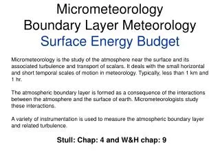
Micrometeorology Surface Layer Dynamics and Surface Energy Exchange

MicrometeorologySurface Layer Dynamics and Surface Energy Exchange Janet Barlow and Andrew Ross

Aims of exercise Micrometeorology is concerned with: • Interaction of atmosphere with the surface • Turbulent mixing • Exchanges of momentum, heat, moisture…traces gases, aerosol • Radiative energy exchange at the surface • Solar (shortwave) • Infra-red (longwave)

Measuring the boundary layer • Boundary Layer • Lowest part of troposphere • Few 10s of metres to ~2km deep • Interacts directly with surface: • Feels the effect of friction • Heated/cooled by surface • Dynamics are dominated by turbulence • Exhibits large diurnal changes in many properties: depth, temperature…

Temperature Profile April 24 2004 stratosphere temperatureinversion boundary layer tropopause free troposphere

Humidity Profile tropopause inversion

Friction: mechanical generation of turbulence Flow over rough surface / obstacles Small perturbations of the flow act as obstacles to the surrounding flow Shear in the flow can result in instability & overturning Turbulence results in a wind speed profile that is close to logarithmic Sources of Turbulence z Wind speed

Convection: heating of air near the surface (or cooling of air aloft) increases (decreases) its density with respect to the air around it, so that it becomes buoyant.

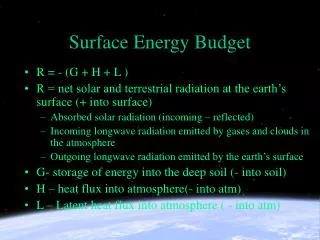
Surface energy budget • Radiative transfer at the Earth’s surface dominates the production or suppression of turbulence in low wind conditions • The heating of the lower layers of the atmosphere is governed by • Heating of the surface itself • Transfer of heat from the surface to the air by four processes: • Absorption and emission of “natural” EM radiation at the surface • Thermal conduction of heat energy within ground • Turbulent transfer of heat energy within the atmosphere • Evaporation of water stored in the surface layer or condensation of water vapour onto surface

Net radiation Flux densities = rate of transfer of energy across a surface Rn Shortwave radiation Latent heat flux Sensible heat flux Longwave radiation LE H Ln=L↓-L↑ Sn= S↓- S↑ = (1-α)S↓ Ground Heat flux G

Surface energy balance • Considering a thin layer of soil at the surface: Heat storage = What goes in - what goes out! For an infinitely thin layer – no heat storage therefore Rn-G=H+LE Where Rn = Sn+Ln

Ultimate aim of SEE/SLD sessions • There are 3 ways of determining H, the sensible heat flux 3. Turbulent eddy measurements Measure heat flux due to turbulent eddies using sonic anemometer data 1. SEE Measure Rn and G Estimate LE from met measurements using Penman-Monteith equation Residual is H (assuming infinitely thin layer) 2. T profile Take a logarithmic T profile from the mast Find friction velocity and friction temperature

SEE Activity • Real-time calculation of radiation budget (using portable mast) Estimates of surface albedo, emissivity, response time 2. Components of the surface energy budget for a time period, and link to meteorology (uses Excel worksheets extensively) 3. Estimate H

Pyranometer Measures the flux of solar radiation (W m-2) Two instruments mounted back to back – measurement of downwelling and upwelling radiation Instruments

Pyrgeometer Measures flux of infrared radiation (W m-2)

Weather station and ground heat flux Ground heat flux is also measured using a plate buried below the ground. Weather station data is used to estimate LE using the Penman-Monteith method. H can be estimated by balancing the budget!

SLD 1 - T profile method • Calculate and analyse temperature and wind profiles from the mast data for two one hour periods (one stable and one unstable). Use these to calculate H • A standard result: under neutral conditions, surface layer winds and temperatures have a logarithmic form. • H can be estimated using the values of u* and T*

Instruments 15m Mast • Air temperature and wind speed are measured at 6 levels on the mast • Also have soil temperature just below surface.

Key parts of SLD1 • Check offset correction is applied • Plot timeseries of quantities to find a stable and unstable period • Plot logarithmic profiles of u and T to find u* and T* • Calculate H

3-D air motion is broken down into 3 velocity components (all in m s-1): u horizontal, along mean wind direction, positive in direction of mean wind v horizontal, perpendicular to u, positive to left of mean wind direction. w vertical, positive upwards w v u

Eddy averaging • Any quantity can be divided into mean and fluctuating terms: • To look at turbulent fluxes we are most concerned with the fluctuating terms e.g. w’

Turbulent fluxes result from the physical movement of parcels of air with different properties: temperature, humidity, gas concentration, momentum… Heat flux Momentum flux Eddy mixes some air down & some air up  w’ -ve w’ +ve Z (m) Z (m) Faster moving air is moved down, slower air is moved up Warmer air is moved upcooler air is moved down 0 Wind speed (m s-1)  (K)

SLD 2 - Turbulent Eddy Measurements • Use sonic anemometer data to calculate surface heat flux • Sonic Anemometer • Measures 3D wind components at very short intervals.

Key parts of SLD2 • Calculate u’ and w’ series from 15 minute sonic measurements • Calculate vertical momentum flux • Calculate u* and H • Compare with T profile measurements

Summary • The SEE and SLD are linked exercises in which you will use different methods to explore the surface layer. • The three experiments will all estimate the value of H, the turbulent transfer of heat energy from the surface to the lower layers of the atmosphere. • You should assess the quality and reliability of the different techniques and what the changing value of H tells you about the meteorological situation.

um wm Sonic axes tilted off vertical  u w = 0

wt ut wm um 

For example, the wind stress at the surface (the vertical flux of horizontal momentum) is • where  is air density, and U the wind speed. • More strictly it is • where u is the wind component in the direction of the mean wind direction and v the component perpendicular to the mean wind. • The wind stress is often represented by the friction velocity

The turbulent flux of some quantity ‘x’ is determined by averaging the vertical exchange of parcels of air with different values of ‘x’. Flux of x = 1 (w′1x′1 + w′2x′2 + …w′Nx′N) N = w′x′ where w′N = wN – w and an overbar signifies averaging

Micrometeorology Surface Layer Dynamics and Surface Energy Exchange