Download
1 / 1
10 likes | 132 Views
UC-Irvine. 3. 8. 7. 4. Spatial and Temporal Resolution Tradeoffs. Hydraulics Model (LISFLOOD-FP). Simulated Interferometric Altimeter Swaths. NASA/JPL Instrument Simulator. Simulated Surface Water Extent and Elevation. Hydrologic Model (VIC). Simulated Stream flow. UW. JPL. U Bristol.

E N D
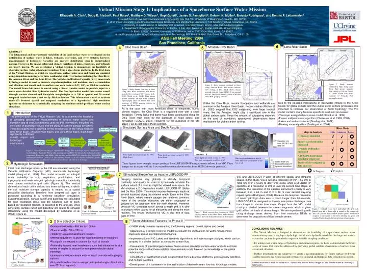
UC-Irvine 3 8 7 4 Spatial and Temporal Resolution Tradeoffs Hydraulics Model (LISFLOOD-FP) Simulated Interferometric Altimeter Swaths NASA/JPL Instrument Simulator Simulated Surface Water Extent and Elevation Hydrologic Model (VIC) Simulated Stream flow UW JPL U Bristol Back Calculation of Discharge UC-Irvine 1 Introduction 5 6 2 Virtual Mission Stage I: Implications of a Spaceborne Surface Water Mission Elizabeth A. Clark1, Doug E. Alsdorf2, Paul Bates3, Matthew D. Wilson4, Gopi Goteti5, James S. Famiglietti5, Delwyn K. Moller6, Ernesto Rodriguez6, and Dennis P. Lettenmaier1 1. Department of Civil and Environmental Engineering, Box 352700, University of Washington, Seattle, WA 98195 2. Ohio State University Department of Geological Sciences, 275 Mendenhall Laboratory, 125 South Oval Mall, Columbus, OH 43210 3. University of Bristol School of Geographical Sciences, University Road, Bristol, BS8 1SS United Kingdom 4. Department of Geography, University of Exeter, 3.046 UEC Tremough, Exeter, EX4 4RJ United Kingdom 5. Earth System Science, University of California, Irvine, 3317 Croul Hall, Irvine, CA 92697 6. Jet Propulsion Laboratory/California Institute of Technology, MS 300-319 4800 Oak Grove Dr., Pasadena, CA 91109 AGU Fall Meeting, 2004San Francisco, California Lena River Basin Amazon River Basin Ohio River Basin ABSTRACT The interannual and interseasonal variability of the land surface water cycle depend on the distribution of surface water in lakes, wetlands, reservoirs, and river systems; however, measurements of hydrologic variables are sparsely distributed, even in industrialized nations. Moreover, the spatial extent and storage variations of lakes, reservoirs, and wetlands are poorly known. We are developing a Virtual Mission to demonstrate the feasibility of observing surface water extent and variations from a spaceborne platform. In the first stage of the Virtual Mission, on which we report here, surface water area and fluxes are emulated using simulation modeling over three continental scale river basins, including the Ohio River, the Amazon River and the Lena River. The Variable Infiltration Capacity (VIC) macroscale hydrologic model is used to simulate evapotranspiration, soil moisture, snow accumulation and ablation, and runoff and streamflow over each basin at 1/8°, 1/2°, or 100-km resolution. The runoff from this model is routed using a linear transfer model to provide input to a much more detailed flow hydraulics model. The flow hydraulics model then routes runoff through various channel and floodplain morphologies at a 250 m spatial and 20 second temporal resolution over a 100 km by 500 km domain. This information is used to evaluate trade-offs between spatial and temporal resolutions of a hypothetical high resolution spaceborne altimeter by synthetically sampling the resultant model-predicted water surface elevations. Figure 7. Study domain (outlined in blue) along Lena River. Red arrows indicate flow routing at 100 km (Su et al., 2004). Green dots show locations of R-Arctic Net gauging locations. Figure 6. Study domain (outlined in blue) along Amazon River. Red arrows indicate flow routing at 1/2°. Black shows stream network derived from SRTM 30 arc-second data set. Green dots show locations of RivDis and GRDC gauging stations. Figure 5. Study domain (outlined in blue)along Ohio River mainstem Red arrows indicate flow routing at 1/8° (Maurer et al., 2002; Wood et al., 2002). Blue shows stream network derived from National Hydrography Data set. Green dots show locations of USGS gauging stations in upper Ohio River Basin. • Due to the possible implications of freshwater inflows to the Arctic Ocean for global climate and the unique arctic surface processes, it is important to increase our observation of Arctic hydrology. The VIC model contains many features specific to cold-land processes: • Two-layer energy balance snow model (Storck et al. 1999) • Frozen soil/permafrost algorithm (Cherkauer et al. 1999, 2003) • Lakes and wetlands model (Bowling et al. 2002) • Blowing snow algorithm (Bowling et al. 2004) Unlike the Ohio River, riverine floodplains and wetlands are common in the Amazon River Basin. Recent studies (Richey et al., 2002) suggest that CO2 outgassing from large tropical rivers, like the Amazon, might play a significant role in the global carbon cycle. Since the amount of outgassing depends on the area of inundation, spaceborne observations have implications for global carbon cycling. As is the case with most American rivers in temperate, humid climate regions, the Ohio River is a regulated river with a small floodplain. Twenty locks and dams have been constructed along the Ohio River main stem for the purposes of flood control and navigation (USACE, 2004). However, for the purposes of the VM stage I, we do not model these controls. The primary goal of the Virtual Mission (VM) is to examine the feasibility of collecting spaceborne measurements of surface water extent and elevation and to evaluate potential uses for this information, including the derivation of discharge values and the study of surface storage dynamics. Three test basins were selected for the initial phase of the Virtual Mission: Ohio River Basin, Amazon River Basin, and Lena River Basin. Each basin Simulated Surface Area and Depth Results represents a different climate region and hydrologic environment. Figure 1. Virtual Mission Stage I experimental design. The hydrologic model component is described here. Bates and Wilson (this meeting section H22C-06) discuss the hydraulics model component. Rodriguez and Moller (this meeting section H22C-08) describe the NASA/JPL Instrument Simulator. Goteti et al. (this meeting section H22C-07) discuss preliminary results regarding spatial and temporal resolution tradeoffs and calculation of discharge. Water depth and extent on Jan. 21, 1995. (High flows). Water depth and extent on April 4, 1995. (Low flows). Water depth and extent on Jan. 21, 1995. This view corresponds to red box at left. Water depth and extent on April 4, 1995. This view corresponds to red box at left. These figures show example images produced from LISFLOOD-FP using dynamic inflows from VIC. These images are in accord with the 1 arc-second resolution elevation data from SRTM (shown in grayscale). Hydrologic Simulation Initial river discharge inputs to the VM are simulated using the Variable Infiltration Capacity (VIC) macroscalehydrologic model (Liang et al., 1994). This model accounts for sub-grid scale variability in soil, vegetation, precipitation, and topography and treats sub-grid hydrologic variability statistically over coarse resolution grid cells (Figure 1). The vertical dimension of each cell is divided into three soil layers, in which the soil moisture storage capacity is treated as a spatial probability distribution. Baseflow from deepest soil layer is produced according to a nonlinear baseflow formulation. Evapotranspiration, surface runoff and baseflow are calculated for each vegetation class, and the weighted sum of each, based on vegetation fraction, is assigned to the grid cell. Once generated, surface runoff and baseflow are routed to simulate streamflow using the model developed by Lohmann et al. (1998; Figure 2). Complete In Progress Simulated Streamflow as Input to LISFLOOD-FP VIC and LISFLOOD-FP work at different spatial and temporal scales. In this study,VIC is run at a resolution of 1/8° (~55 km) to 1000 km over 3-hourly to daily time steps, while LISFLOOD-FP operates at a resolution of 270 m over 20-second time steps. In addition, the resolution of the satellite instrument is likely to vary between 2 m x 60 m and 2 m x 10 m over several day-long repeat cycles (Rodriguez, 2004). Because the temporal resolution of most hydrologic data sets is much longer than 20-seconds, LISFLOOD-FP is designed to linearly interpolate discharge data from longer to shorter time steps. Output from the VIC model routing is divided between the stream segments within a given grid cell on the basis of stream length. We are experimenting with using drainage areas derived from finer resolution DEMs to determine the proportions of flow to each stream. Gauging stations vary globally in density, temporal continuity, and quality. In order to dynamically simulate the surface extent of a river as might be viewed from space, the VM employs a 2-D hydraulics model, LISFLOOD-FP (Bates and De Roo, 2000). This model requires hydrologic inputs at several locations along the channel reach. Even in the Ohio River Basin, where stream gauges are relatively common, many of the smaller tributaries are either ungauged or gauged too far upstream from the main channel. However, because VIC simulates runoff across a mesh grid, it is able to produce inflow values for all tributaries and along the main reaches. The record produced by VIC is also free of data gaps in time. Figure 4. Colored boxes show individual VIC grid cells. Runoff from all of these cells is routed to the orange cell. This cell contains three outflow points (green), so the flow assigned to each point is the flow entering the green cell weighted by the length of river upstream of each point. Figure 1. Schematic representation of VIC hydrologic model. Figure 3. Black crosses show location of USGS gauging stations in the Ohio River study domain. Red dots show the desired locations of flow inputs. Some Additional Features for Phase II Site Selection Criteria • Domain size ideally ~500 km by 100 km • Channel width ~50 to 200 m • Relatively straight mainstream reaches • Minimal regulation: to allow for natural flooding in tributaries • Floodplain connected to channel for most of domain • Preferably located near headwaters such that tributaries lie at a variety of angles to account for non-perpendicular orbital crossings • Upstream and downstream ends of reach coincide with gauging stations • Not parallel with orbital crossings (anticipated angle of inclination near 65° from equator) • 3 NEW study domains representing the following regions: boreal, alpine and desert. • Application of a simple reservoir model to evaluate the implications for water management, especially across international boundaries. • Implementation of VIC Lakes and Wetlands algorithm to estimate storage changes, which can be sampled in a similar fashion as simulated stream flow. • Calculations of typical biogeochemical fluxes across simulated surface water areas to estimate potential impacts that these satellite measurements could have on our knowledge of the global carbon cycle. • Simulations of swaths that would be generated from sub-orbital platforms, geostationary satellites, and multiple satellites. • Development of a framework for the assimilation of derived stream flow into hydrologic models. CONCLUDING REMARKS • The Virtual Mission is designed to demonstrate the feasibility of a spaceborne surface water observation system. It employs a hydrologic model and a hydraulics model to discharge and surface extent that can then be perturbed to represent variable sampling conditions. • By testing over a wide range of hydrologic and climate regions, we hope to demonstrate the broad scope of issues that could be addressed by providing global satellite observations of surface water extent and elevation. • Further investigations are underway to create a recommendation for future surface hydrology satellite missions that would account for tradeoffs in spatial and temporal data collection resolution. Figure 2. Schematic representation of routing model. Authors would like to thank Ed Maurer at UC Santa Clara, Andrew Wood, Fengge Su, and Jennifer Adam at University of Washington.