Download
1 / 23
680 likes | 1.99k Views
Flow Nets. Prepared By: Eng. Hayder M. Jasem AL- Mosawey Supervisor : Dr. Mohamed Shaker. Flow Net Theory. Streamlines Y and Equip. lines are . Streamlines Y are parallel to no flow boundaries. Grids are curvilinear squares, where diagonals cross at right angles.

E N D
Flow Nets Prepared By: Eng. Hayder M. Jasem AL- Mosawey Supervisor : Dr. Mohamed Shaker
Flow Net Theory • Streamlines Y and Equip. lines are . • Streamlines Y are parallel to no flow boundaries. • Grids are curvilinear squares, where diagonals cross at right angles. • Each stream tube carries the same flow.
Flow Net in Isotropic Soil Portion of a flow net is shown below Y Stream tube F
Flow Net in Isotropic Soil • The equation for flow nets originates from Darcy’s Law. • Flow Net solution is equivalent to solving the governing equations of flow for a uniform isotropic aquifer with well-defined boundary conditions.
Flow Net in Isotropic Soil • Flow through a channel between equipotential lines 1 and 2 per unit width is: ∆q = K(dm x 1)(∆h1/dl) n F1 m F2 Dq F3 Dq Dh1 Dh2 dm dl
Flow Net in Isotropic Soil • Flow through equipotential lines 2 and 3 is: ∆q = K(dm x 1)(∆h2/dl) • The flow net has square grids, so the head drop is the same in each potential drop: ∆h1 = ∆h2 • If there are nd such drops, then: ∆h = (H/n) where H is the total head loss between the first and last equipotential lines.
Flow Net in Isotropic Soil • Substitution yields: • ∆q = K(dm/dl)(H/n) • This equation is for one flow channel. If there are m such channels in the net, then total flow per unit width is: • q = (m/n)K(dm/dl)H
Flow Net in Isotropic Soil • Since the flow net is drawn with squares, then dm dl, and: q = (m/n)KH [L2T-1] where: • q = rate of flow or seepage per unit width • m= number of flow channels • n= number of equipotential drops • h = total head loss in flow system • K = hydraulic conductivity(Permeability)
Drawing Method: 1. Draw to a convenient scale the cross sections of the structure, water elevations, and aquifer profiles. 2. Establish boundary conditions and draw one or two flow lines Y and equipotential lines F near the boundaries.
Drawing Method: 3. Sketch intermediate flow lines and equipotential lines by smooth curves adhering to right-angle intersections and square grids. Where flow direction is a straight line, flow lines are an equal distance apart and parallel. 4. Continue sketching until a problem develops. Each problem will indicate changes to be made in the entire net. Successive trials will result in a reasonably consistent flow net.
Method: • In most cases, 5 to 10 flow lines are usually sufficient. Depending on the no. of flow lines selected, the number of equipotential lines will automatically be fixed by geometry and grid layout. 6. Equivalent to solving the governing equations of GW flow in 2-dimensions.
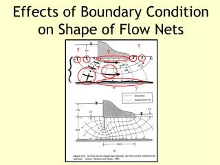
Seepage Under Dams Flow nets for seepage through earthen dams Seepage under concrete dams Uses boundary conditions (L & R) Requires curvilinear square grids for solution
Two Layer Flow System with Sand Below Ku / Kl = 1 / 50
Two Layer Flow System with Tight Silt Below Flow nets for seepage from one side of a channel through two different anisotropic two-layer systems. (a) Ku / Kl = 1/50. (b) Ku / Kl = 50.. Source: Todd & Bear, 1961
Radial Flow: Contour map of the piezometric surface near Savannah, Georgia, 1957, showing closed contours resulting from heavy local groundwater pumping (after USGS Water-Supply Paper 1611).
Flow Net in a Corner: Streamlines Y are at right angles to equipotential F lines
Flow Nets: an example • A dam is constructed on a permeable stratum underlain by an impermeable rock. A row of sheet pile is installed at the upstream face. If the permeable soil has a hydraulic conductivity of 150 ft/day, determine the rate of flow or seepage under the dam.
Flow Nets: an example The flow net is drawn with: m = 5 n = 17
Flow Nets: the solution • Solve for the flow per unit width: q = (m/n) K h = (5/17)(150)(35) = 1544 ft3/day per ft
Flow Nets: An Example • There is an earthen dam 13 meters across and 7.5 meters high.The Impounded water is 6.2 meters deep, while the tail water is 2.2 meters deep. The dam is 72 meters long. If the hydraulic conductivity is 6.1 x 10⁻⁴ centimeter per second, what is the seepage through the dam if n = 21 K = 6.1 x 104cm/sec = 0.527 m/day
Flow Nets: the solution • From the flow net, the total head loss, H, is 6.2 -2.2 = 4.0 meters. • There are 6 flow channels (m) and 21 head drops along each flow path (n): Q = (KmH/n) x dam length = (0.527 m/day x 6 x 4m / 21) x (dam length) = 0.60 m3/day per m of dam • = 43.4 m3/day for the entire 72-meter length of the dam