Download
1 / 24
240 likes | 345 Views
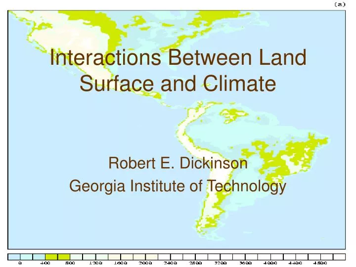
Interactions Between Land Surface and Climate. Robert E. Dickinson Georgia Institute of Technology. Overall System Description. d ψ /dt = f (ψ, λ, t ) , (1) ψ = state of everything in climate system λ = externally specified parameters.

E N D
Interactions Between Land Surface and Climate Robert E. Dickinson Georgia Institute of Technology
Overall System Description d ψ /dt = f (ψ, λ, t ) , (1) ψ = state of everything in climate system λ = externally specified parameters. We are forced to view this system in probabilistic terms for 2-related reasons: • Its observational description at time t has to be probabilistic. • It has about 10 29 degrees of freedom but we can integrate deterministically about 10 9.
What should probabilistic generally not mean (can be useful shortcuts but should nog be long satisfied with)? • Smashing everything into Gaussians • Expressing all small scale effects as covariances tied to large scale as eddy diffusion. • Conceptualizing small scale processes as 1-D column exchange processes that we hope will mimic the real 3-D processes. • Adding time correlated noise (i.e. Markov + Wiener process) forcing
What should probabilistic mean? • Thoughtful attention to how to sum up from small scale to that resolved by model, by making the descriptions of small scale realistic on the scale they represent and then devising means to sum them up. • Need to identify all the summary variables that couple to large scale – covariances are obvious but what else? How do different scales below that resolved enter in?
Schematic of Interacting Climate System (redrafted interpretation of plots in IPCC-2001)
Relevance to Land Surface and Climate? • Land processes are conceptualized on scale of 1 to 10 3 m. • Global observational information available to finer than 1 km. • Much of the coupling of atmosphere to land occurs on scales unresolved by model mesh • Many of the anthropogenic disturbances to land occur on a small scale – not obvious how to add their effects
One of many possible examples CLM land model has largely not yet addressed scaling issues: The occurrence of most convective precipitation on scale small compared to that resolved may have consequences – what are they? Control is application of precipitation uniformly over a grid square – more realistic is express it as a pdf – how?
Atmospheric Model Precipitation Atmospheric model now make precipitation to provide its need for diabatic heating and to provide the land and ocean model a volume fresh water input. The land model, however, needs additional statistical information that it currently cannot get from the atmosphere, so it has to be satisfied with a “second” best use of observational constraints.
Exponential Distribution P(x) If x a random variable distributed randomly, its pdf is: P(x) = (1./ [x] )exp(-x/[x]), where brackets denote expected value. The simplest description of precipitation over land requires two variables: a) the fractional area over which it rains Ap; b) the distribution of intensities over which the rain occurs. These are estimated each time step through application of two control variables: an over all expected intensity [P] and an auto-correlation time t. The term Ap is exponentially distributed with expected value given by the ratio of grid square average divided by [P]. Over this area, the intensity is also distributed using [P], with areas of past rain continuing from autocorrelation
Implementation • Run with CAM 2.2 + CLM2.2 = CAM 3 + CLM3. • 4 test cases: divide grid cell into 10 or 30 elements (+some further details) • Largest effects are expected with tropical precip so tailored to that. • Impose base rate for P of 5 mm/hr. It is reduce by cos (sun angle) for local noon, to make more reasonable for high latitudes
Some Conclusions – re Amazon • Frequency of tropical rainfall decreased by order of magnitude (intensities so increase) • Water evaporated by canopy reduces by factor to two – transpiration like increases • Some increase of runoff – especially in dry season • Some increase of surface radiation – overall somewhat warmer and drier – more sensible • Average of P and E change little
So what? • Changes time scales of soil moisture variability and coupling to ET. • Carbon assimilation driven by transpiration so want to get rid of such serious bias.
Land model key framework for modeling carbon. • Describes the local micrometeorological drivers of carbon cycling: T’s of canopy and soil, transpiration, PAR (direct and diffuse), surface turbulence. • Drives the convective transports that are a major contributor to CO2 distribution. • Carbon community assumes the existence of a transport model to move C in atmosphere – little realization that such one of the weakest parts of what is is conceptually they want to do. Also a weak area of climate modeling in general
How to learn more about atmospheric transport by study of tracer redistributions? • Obviously not a new idea – but so far success has been limited. • New conceptual and observational tools should make easier. • Satellites give global measurements of tracers • EnKF gives a much superior tool for satellite data assimilation.
What can be done? • Ensemble simulations give simple way to estimate covariances – getting such appears to have been one of the biggest obstacles to more rapid incorporation of new measurements – earlier approaches such as 4-D var need to construct adjoint models and need to predict full covariance terms.
How to use tracers? • Standard problem: given measurement y, compare forward calculation from model state x with h(x) • Easy to relate optimally and linearly h(x) to x using regression with ensemble (Jeff Anderson, 2003). • Calculate satellite radiances from modeled tracer – correlations over ensemble give not only measurement of tracer but also of wind – need 2 tracers to get vector – since variability of tracers largely controlled by atmospheric transport, this should be a really useful analysis (maybe better than LAWS?) – messed up by small scale but also want to learn about that anyway. • Maybe SVDs of correlation matrix optimum low D basis?
Concluding Remarks • Land is key ingredient of climate system • Need more advanced probabilistic framework to better link to atmosphere • Coupling to atmospheric convective processes needs to be better described for a variety of important climate system objectives.